Spin Hamiltonians in Magnets: Theories and Computations
磁体中的自旋哈密顿量：理论与计算

Abstract  摘要

The effective spin Hamiltonian method has drawn considerable attention for its power to explain and predict magnetic properties in various intriguing materials. In this review, we summarize different types of interactions between spins (hereafter, spin interactions, for short) that may be used in effective spin Hamiltonians as well as the various methods of computing the interaction parameters. A detailed discussion about the merits and possible pitfalls of each technique of computing interaction parameters is provided.
有效自旋哈密顿量方法因其解释和预测各种有趣材料磁性质的能力而受到广泛关注。在本综述中，我们总结了可用于有效自旋哈密顿量中的不同类型的自旋相互作用（以下简称自旋相互作用）以及计算相互作用参数的各种方法。对计算相互作用参数每种技术的优缺点进行了详细讨论。

1. Introduction  1. 引言

The utilization of magnetism can date back to ancient China when the compass was invented to guide directions. Since the relationship between magnetism and electricity was revealed by Oersted, Lorentz, Ampere, Faraday, Maxwell, and others, more applications of magnetism have been invented, which include dynamos (electric generators), electric motors, cyclotrons, mass spectrometers, voltage transformers, electromagnetic relays, picture tubes, and sensing elements. During the information revolution, magnetic materials were extensively employed for information storage. The storage density, efficiency, and stability were substantially improved by the discovery and applications of the giant magnetoresistance effect [1,2], tunnel magnetoresistance [3,4,5,6,7,8,9], spin-transfer torques [10,11,12,13], etc. Recently, more and more novel magnetic states such as spin glasses [14,15], spin ice [16,17], spin liquid [18,19,20,21,22], and skyrmions [23,24,25,26,27,28] were found, revealing both theoretical and practical significance. For example, hedgehogs and anti-hedgehogs can be seen as the sources (monopoles) and the sinks (antimonopoles) of the emergent magnetic fields of topological spin textures [29], while magnetic skyrmions have shown promise as ultradense information carriers and logic devices [24].
磁性利用可以追溯到古代中国，当时发明指南针来指引方向。自从奥斯特、洛伦兹、安培、法拉第、麦克斯韦等人揭示了磁性与电之间的关系以来，磁性的更多应用被发明出来，包括发电机（电动机）、电动机、回旋加速器、质谱仪、电压变压器、电磁继电器、显像管和传感元件等。在信息革命期间，磁性材料被广泛用于信息存储。通过发现和应用巨磁阻效应[1, 2]、隧道磁阻[3, 4, 5, 6, 7, 8, 9]、自旋转移扭矩[10, 11, 12, 13]等，存储密度、效率和稳定性得到了显著提高。最近，发现了越来越多的新型磁性状态，如自旋玻璃[14, 15]、自旋冰[16, 17]、自旋液体[18, 19, 20, 21, 22]和磁 Skyrmions[23, 24, 25, 26, 27, 28]，这既具有理论意义，也具有实际意义。 例如，刺猬和反刺猬可以被视为拓扑自旋纹理中涌现磁场的源（单极子）和汇（反单极子）[29]，而磁 Skyrmions 已显示出作为超密集信息载体和逻辑器件的潜力[24]。

To explain or predict the properties of magnetic materials, many models and methods have been invented. In this review, we will mainly focus on the effective spin Hamiltonian method based on first-principles calculations, and its applications in solid-state systems. In Section 2, we will introduce the effective spin Hamiltonian method. Firstly, in Section 2.1, the origin and the computing methods of the atomic magnetic moments are presented. Then, from Section 2.2, Section 2.3, Section 2.4, Section 2.5 and Section 2.6, different types of spin interactions that may be included in the spin Hamiltonians are discussed. Section 3 will discuss and compare various methods of computing the interaction parameters used in the effective spin Hamiltonians. In Section 4, we will give a brief conclusion of this review.
为了解释或预测磁性材料的性质，已经发明了许多模型和方法。在本综述中，我们将主要关注基于第一性原理计算的有效自旋哈密顿量方法及其在固态系统中的应用。在第 2 节中，我们将介绍有效自旋哈密顿量方法。首先，在第 2.1 节中，将介绍原子磁矩的起源和计算方法。然后，从第 2.2 节到第 2.6 节，将讨论可能包含在自旋哈密顿量中的不同类型的自旋相互作用。第 3 节将讨论和比较用于有效自旋哈密顿量的相互作用参数的计算方法。在第 4 节中，我们将对本综述给出简要结论。

2. Effective Spin Hamiltonian Models
2. 有效自旋哈密顿量模型

Though accurate, first-principles calculations are somewhat like black boxes (that is to say, they provide the final total results, such as magnetic moments and the total energy, but do not give a clear understanding of the physical results without further analysis), and have difficulties in dealing with large-scale systems or finite temperature properties. In order to provide an explicit explanation for some physical properties and improve the efficiency of thermodynamic and kinetic simulations, the effective Hamiltonian method is often adopted. In the context of magnetic materials where only the spin degree of freedom is considered, it can also be called the effective spin Hamiltonian method. Typically, the effective spin Hamiltonian models need to be carefully constructed and include all the possibly important terms; then the parameters of the models need to be calculated based on either first-principles calculations (see Section 3) or experimental data (see Section 3.3). Given the effective spin Hamiltonian and the spin configurations, the total energy of a magnetic system can be easily computed. Therefore, it is often adopted in Monte Carlo simulations [30] (or quantum Monte Carlo simulations) for assessing the total energy of many different configurations so that the finite temperature properties of magnetic materials can be studied. If the effects of atom displacements are taken into account, the effective Hamiltonians can also be applied to the spin molecular dynamics simulations [31,32,33], which is beyond the scope of this review.
尽管准确，但基于第一性原理的计算有点像黑箱（也就是说，它们提供了最终的总结果，如磁矩和总能量，但如果没有进一步的分析，则无法清楚地理解物理结果），并且在处理大规模系统或有限温度性质时存在困难。为了对某些物理性质提供明确的解释并提高热力学和动力学模拟的效率，通常采用有效哈密顿量方法。在仅考虑磁材料中自旋自由度的背景下，这也可以称为有效自旋哈密顿量方法。通常，需要仔细构建有效自旋哈密顿量模型并包括所有可能的重要项；然后，需要根据第一性原理计算（见第 3 节）或实验数据（见第 3.3 节）计算模型参数。给定有效自旋哈密顿量和自旋配置，可以轻松计算磁系统的总能量。 因此，它通常被用于蒙特卡洛模拟[30]（或量子蒙特卡洛模拟）中，以评估许多不同配置的总能量，从而研究磁性材料的有限温度性质。如果考虑原子位移的影响，有效哈密顿量也可以应用于自旋分子动力学模拟[31, 32, 33]，这超出了本综述的范围。

In this review, we mainly focus on the classical effective spin Hamiltonian method where atomic magnetic moments (or spin vectors) are treated as classical vectors. In many cases, these classical vectors are assumed to be rigid so that their magnitudes keep constant during rotations. This treatment significantly simplifies the effective Hamiltonian models, and it is usually a good approximation, especially when atomic magnetic moments are large enough.
在这篇综述中，我们主要关注经典有效自旋哈密顿量方法，其中原子磁矩（或自旋矢量）被处理为经典矢量。在许多情况下，这些经典矢量被假定为刚性的，因此它们的幅度在旋转过程中保持不变。这种处理显著简化了有效哈密顿量模型，并且通常是一个很好的近似，尤其是在原子磁矩足够大时。

In this part, we shall first introduce the origin of the atomic magnetic moments as well as the methods of computing atomic magnetic moments. Then different types of spin interactions will be discussed.
在这一部分，我们将首先介绍原子磁矩的起源以及计算原子磁矩的方法。然后，将讨论不同类型的自旋相互作用。

2.1. Atomic Magnetic Moments
2.1. 原子磁矩

The origin of atomic magnetic moments is explained by quantum mechanics. Suppose the quantized direction is the z-axis, an electron with quantum numbers (𝑛, 𝑙 ,𝑚𝑙, 𝑚𝑠$n, l ,m_l, m_s$) leads to an orbital magnetic moment 𝝁𝑙= −𝜇𝐵𝒍${\mathit{\mu }}_l= -{\mu }_B\mathit{l}$ and a spin magnetic moment 𝝁𝑠= −𝑔𝑒𝜇𝐵𝒔${\mathit{\mu }}_s= -g_e{\mu }_B\mathit{s}$, with their z components 𝜇𝑙𝑧= −𝑚𝑙𝜇𝐵${\mu }_{lz}= -m_l{\mu }_B$ and 𝜇𝑠𝑧= −𝑔𝑒𝑚𝑠𝜇𝐵${\mu }_{sz}= -g_e{m}_s{\mu }_B$, where 𝜇𝐵= |𝑒|ℏ2𝑚${\mu }_B= \frac{\left|e\right|\hslash }{2m}$ is the Bohr magneton and 𝑔𝑒≈2$g_e\approx 2$ is the g-factor for a free electron. The energy of a magnetic moment 𝝁$\mathit{\mu }$ in a magnetic field 𝑩$\mathit{B}$ (magnetic induction) along z-direction is −𝝁⋅𝑩 = −𝜇𝑧𝐵$-\mathit{\mu }\cdot \mathit{B} = -{\mu }_{z}B$.
原子磁矩的起源由量子力学解释。假设量子化的方向是 z 轴，具有量子数（ 𝑛, 𝑙 ,𝑚𝑙, 𝑚𝑠$n, l ,m_l, m_s$ ）的电子导致轨道磁矩 𝝁𝑙= −𝜇𝐵𝒍${\mathit{\mu }}_l= -{\mu }_B\mathit{l}$ 和自旋磁矩 𝝁𝑠= −𝑔𝑒𝜇𝐵𝒔${\mathit{\mu }}_s= -g_e{\mu }_B\mathit{s}$ ，它们的 z 分量分别为 𝜇𝑙𝑧= −𝑚𝑙𝜇𝐵${\mu }_{lz}= -m_l{\mu }_B$ 和 𝜇𝑠𝑧= −𝑔𝑒𝑚𝑠𝜇𝐵${\mu }_{sz}= -g_e{m}_s{\mu }_B$ ，其中 𝜇𝐵= |𝑒|ℏ2𝑚${\mu }_B= \frac{\left|e\right|\hslash }{2m}$ 是玻尔磁子， 𝑔𝑒≈2$g_e\approx 2$ 是自由电子的 g 因子。磁矩 𝝁$\mathit{\mu }$ 在沿 z 方向的磁场 𝑩$\mathit{B}$ （磁感应强度）中的能量是 −𝝁⋅𝑩 = −𝜇𝑧𝐵$-\mathit{\mu }\cdot \mathit{B} = -{\mu }_{z}B$ 。

Considering the Russell-Saunders coupling (also referred to as L-S coupling), which applies to most multi-electronic atoms, the total orbital magnetic moment and the total spin magnetic moment are 𝝁𝐿= −𝜇𝐵𝑳${\mathit{\mu }}_L= -{\mu }_B\mathit{L}$ and 𝝁𝑆= −𝑔𝑒𝜇𝐵𝑺${\mathit{\mu }}_S= -g_e{\mu }_B\mathit{S}$, respectively, where 𝑳 = ∑𝑖𝒍𝑖$\mathit{L} = {\displaystyle \sum }_i{\mathit{l}}_i$ and 𝑺 = ∑𝑖𝒔𝑖$\mathit{S} = {\displaystyle \sum }_i{\mathit{s}}_i$ are the summation over electrons. The quantum numbers of each electron can usually be predicted by Hund’s rules. Owing to the spin–orbit interaction, 𝑳$\mathit{L}$ and 𝑺$\mathit{S}$ both precess around the constant vector 𝑱 = 𝑳+𝑺$\mathit{J} = \mathit{L}+\mathit{S}$. The time-averaged effective total magnetic moment is 𝝁 = −𝑔𝐽𝜇𝐵𝑱$\mathit{\mu } = -g_J{\mu }_B\mathit{J}$, where
考虑到 Russell-Saunders 耦合（也称为 L-S 耦合），它适用于大多数多电子原子，总轨道磁矩和总自旋磁矩分别为 𝝁𝐿= −𝜇𝐵𝑳${\mathit{\mu }}_L= -{\mu }_B\mathit{L}$ 和 𝝁𝑆= −𝑔𝑒𝜇𝐵𝑺${\mathit{\mu }}_S= -g_e{\mu }_B\mathit{S}$ ，其中 𝑳 = ∑𝑖𝒍𝑖$\mathit{L} = {\displaystyle \sum }_i{\mathit{l}}_i$ 和 𝑺 = ∑𝑖𝒔𝑖$\mathit{S} = {\displaystyle \sum }_i{\mathit{s}}_i$ 是电子的求和。每个电子的量子数通常可以通过 Hund 规则预测。由于自旋-轨道相互作用， 𝑳$\mathit{L}$ 和 𝑺$\mathit{S}$ 都围绕常数向量 𝑱 = 𝑳+𝑺$\mathit{J} = \mathit{L}+\mathit{S}$ 进动。时间平均的有效总磁矩为 𝝁 = −𝑔𝐽𝜇𝐵𝑱$\mathit{\mu } = -g_J{\mu }_B\mathit{J}$ ，其中

𝑔𝐽= 1+𝐽(𝐽+1)+𝑆(𝑆+1)−𝐿(𝐿+1)2𝐽(𝐽+1)$$g_J= 1+\frac{J\left(J+1\right)+S\left(S+1\right)-L\left(L+1\right)}{2J\left(J+1\right)}$$

(1)

The atomic magnetic moments discussed above are based on the assumption that the atoms are isolated. Taking the influence of other atoms and external fields into account, the orbital interaction theory, the crystal field theory [34], or the ligand field theory [35,36] may be a better choice for theoretically predicting atomic magnetic moments. Notice that half-filled shells lead to a total 𝑳 = 0$\mathit{L} = 0$, and that in solids and molecules, orbital moments of electrons are usually quenched, resulting in an effective 𝑳 = 0$\mathit{L} = 0$ [37] (counterexamples may be found for 4f elements or for 3d⁷ configurations as in Co(II)). Therefore typically 𝝁 = 𝝁𝑆$\mathit{\mu } = {\mathit{\mu }}_S$, with its z component 𝜇𝑧= −𝑔𝑒𝑆𝑧𝜇𝐵${\mu }_z= -g_e{S}_z{\mu }_B$ (𝑆𝑧$S_z$ is restricted to discrete values: 𝑆, 𝑆−1,…,−𝑆$S, S-1,\dots ,-S$). Usually, a nonzero 𝝁𝑆${\mathit{\mu }}_S$ results from singly filled (localized) d or f orbitals, while s and p orbitals are typically either doubly filled or vacant so that they have no direct contribution to the atomic magnetic moments. Therefore, when referring to atomic magnetic moments, usually only the atoms in the d- and f-transition series need to be considered.
上述讨论的原子磁矩基于原子是孤立的假设。考虑其他原子和外部场的影响，轨道相互作用理论、晶体场理论[34]或配位场理论[35, 36]可能是理论上预测原子磁矩的更好选择。请注意，半充满壳层导致总 𝑳 = 0$\mathit{L} = 0$ ，在固体和分子中，电子的轨道矩通常被淬灭，导致有效的 𝑳 = 0$\mathit{L} = 0$ [37]（对于 4 个元素或如 Co(II)中的 3d ⁷ 配置等可能存在反例）。因此通常 𝝁 = 𝝁𝑆$\mathit{\mu } = {\mathit{\mu }}_S$ ，其 z 分量 𝜇𝑧= −𝑔𝑒𝑆𝑧𝜇𝐵${\mu }_z= -g_e{S}_z{\mu }_B$ （ 𝑆𝑧$S_z$ 被限制为离散值： 𝑆, 𝑆−1,…,−𝑆$S, S-1,\dots ,-S$ ）。通常，非零 𝝁𝑆${\mathit{\mu }}_S$ 来自单占据（局域）d 或轨道，而 s 和 p 轨道通常是双占据或空，因此它们对原子磁矩没有直接贡献。因此，当提到原子磁矩时，通常只需要考虑 d-和-过渡系列的原子。

The atomic magnetic moments can also be predicted numerically employing first-principles calculations. Nevertheless, we should notice that traditional Kohn–Sham density functional theory (DFT) calculations [38,39] (based on single-electron approximation) are not reliable for predicting atomic magnetic moments, and hence require the consideration of strong correlation effect among electrons, especially when dealing with localized d or f orbitals. Based on the Hubbard model [40], such problem can often be remedied by introducing an intra-atomic interaction with effective on-site Coulomb and exchange parameters, U and J [41] (or only one parameter 𝑈eff= 𝑈−𝐽$U^{\mathrm{eff}}= U-J$ in Dudarev’s approach [42]). This approach is the DFT+U method [41,42,43,44], including LDA+U (LDA: Local density approximation), LSDA+U (LSDA: Local spin density approximation), GGA+U (GGA: Generalized gradient approximation), and so forth, where “+U” indicates the Hubbard “+U” correction. The parameters U and J can be estimated according to experience or semi-empirically by seeking agreement with experimental results of some specific properties, which is convenient but not very reliable. Considering how the values of the parameters U and J affect the prediction of atomic magnetic moments and other physical properties, we may need to compute these parameters more rigorously. A typical approach is constrained DFT calculations [43,45,46,47], where the local d or f charges are constrained to different values in several calculations, so that the parameters U and J can be obtained. Another approach based on constrained random-phase approximation (cRPA) [48,49,50] allows for considering the frequency (or energy) dependence of the parameters. More methods of computing U and J are summarized in Ref. [43]. There are more accurate approaches for dealing with strong correlated systems like DFT + Dynamical Mean Field Theory (DFT+DMFT) [51,52,53,54,55] and Reduced Density Matrix Functional Theory (RDMFT) [56,57], but they are much more sophisticated and computationally demanding so that they may be impractical for large-scale calculations. Wave function (WF) methods, such as Complete Active Space Self-Consistent Field (CASSCF) [58,59,60,61], Complete Active Space second-order Perturbation Theory (CASPT2) [62,63,64], Complete Active Space third-order Perturbation Theory (CASPT3) [65], and Difference Dedicated Configuration Interaction (DDCI) [66,67,68], are also widely adopted by theoretical chemists for studying magnetic properties of materials (especially molecules), including atomic magnetic moments and magnetic interactions. These WF methods are also more accurate but more computationally demanding than the DFT+U method, more detailed discussions of which can be found in Ref. [69].
原子磁矩也可以通过第一性原理计算进行数值预测。然而，我们应该注意到，基于单电子近似的传统 Kohn-Sham 密度泛函理论（DFT）计算[38, 39]（基于单电子近似）在预测原子磁矩方面并不可靠，因此需要考虑电子之间的强关联效应，尤其是在处理局域 d 或轨道时。基于 Hubbard 模型[40]，通过引入具有有效局域库仑和交换参数 U 和 J[41]（或 Dudarev 方法中的单一参数 𝑈eff= 𝑈−𝐽$U^{\mathrm{eff}}= U-J$ [42]）的原子内相互作用，此类问题通常可以得到解决。这种方法是 DFT+U 方法[41, 42, 43, 44]，包括 LDA+U（LDA：局域密度近似）、LSDA+U（LSDA：局域自旋密度近似）、GGA+U（GGA：广义梯度近似）等，其中“+U”表示 Hubbard 的“+U”修正。U 和 J 参数可以根据经验或半经验地通过寻求与某些特定性质的实验结果一致来估计，这种方法方便但并不非常可靠。 考虑到参数 U 和 J 的值如何影响原子磁矩和其他物理性质的预测，我们可能需要更严格地计算这些参数。一种典型的方法是受约束的 DFT 计算[43, 45, 46, 47]，在几次计算中将局部 d 或电荷约束到不同的值，从而可以获得 U 和 J 参数。另一种基于受约束随机相近似(cRPA)[48, 49, 50]的方法允许考虑参数的频率（或能量）依赖性。U 和 J 的计算方法更多，总结在参考文献[43]中。对于处理强关联系统（如 DFT + 动态平均场理论(DFT+DMFT)[51, 52, 53, 54, 55]和简化密度矩阵泛函理论(RDMFT)[56, 57]）有更精确的方法，但它们更加复杂且计算需求更高，因此对于大规模计算可能不切实际。 波函数（WF）方法，如完全主动空间自洽场（CASSCF）[58, 59, 60, 61]、完全主动空间二阶微扰理论（CASPT2）[62, 63, 64]、完全主动空间三阶微扰理论（CASPT3）[65]和差分专用配置相互作用（DDCI）[66, 67, 68]，也被理论化学家广泛采用来研究材料的磁性（尤其是分子）性质，包括原子磁矩和磁相互作用。这些波函数方法比 DFT+U 方法更精确，但计算需求也更高，更详细的讨论可以在参考文献[69]中找到。

2.2. Heisenberg Model  2.2. 海森堡模型

The simplest effective spin Hamiltonian model is the classical Heisenberg model, which can be reduced to Ising model or XY model. The classical Heisenberg model can be written as
最简单的有效自旋哈密顿量模型是经典海森堡模型，它可以简化为伊辛模型或 XY 模型。经典海森堡模型可以写成

𝐻𝑠pin = ∑𝑖,𝑗>𝑖𝐽𝑖𝑗𝑺𝑖⋅𝑺𝑗,$$H_{s\mathrm{pin}} = {\displaystyle \sum }_{i,j>i}{J}_{ij}{\mathit{S}}_i\cdot {\mathit{S}}_j,$$

(2)

where 𝑺𝑖${\mathit{S}}_i$ and 𝑺𝑗${\mathit{S}}_j$ indicate the total spin vectors on atoms 𝑖$i$ and 𝑗$j$, and the summation is over all relevant pairs (𝑖𝑗)$\left(ij\right)$. Its form was suggested by Heisenberg, Dirac, and Van Vleck. Such an interaction comes from the energy splitting between quantized parallel (ferromagnetic, FM; triplet state) and antiparallel (antiferromagnetic, AFM; singlet state) spin configurations. 𝐽𝑖𝑗>0$J_{ij}>0$ and 𝐽𝑖𝑗<0$J_{ij}<0$ prefer AFM and FM configurations, respectively. There may be a difference in the factor such as −1 and 12$\frac{1}{2}$ between different definitions of 𝐻𝑠pin$H_{s\mathrm{pin}}$, which is also the case in other models as will be discussed.
其中 𝑺𝑖${\mathit{S}}_i$ 和 𝑺𝑗${\mathit{S}}_j$ 表示原子 𝑖$i$ 和 𝑗$j$ 上的总自旋矢量，求和遍历所有相关对 (𝑖𝑗)$\left(ij\right)$ 。其形式由海森堡、狄拉克和范弗莱克提出。这种相互作用来源于量子化的平行（铁磁，FM；三重态）和反平行（反铁磁，AFM；单态）自旋配置之间的能量分裂。 𝐽𝑖𝑗>0$J_{ij}>0$ 和 𝐽𝑖𝑗<0$J_{ij}<0$ 分别倾向于反铁磁和铁磁配置。 𝐻𝑠pin$H_{s\mathrm{pin}}$ 的不同定义之间可能存在如-1 和 12$\frac{1}{2}$ 这样的因子差异，其他模型中也是如此，将在讨论中说明。

The spatial wave function of two electrons should possess the form of 𝜓± = 12√[𝜓𝑎(𝒓1)𝜓𝑏(𝒓2)±𝜓𝑏(𝒓1)𝜓𝑎(𝒓2)]${\psi }_{\pm } = \frac{1}{\sqrt{2}}\left[{\psi }_a\left({\mathit{r}}_1\right){\psi }_b\left({\mathit{r}}_2\right)\pm {\psi }_b\left({\mathit{r}}_1\right){\psi }_a\left({\mathit{r}}_2\right)\right]$, where 𝜓𝑎${\psi }_a$ and 𝜓𝑏${\psi }_b$ are any single-electron spatial wave functions. A parallel triplet spin state and an antiparallel singlet spin state should correspond to an antisymmetric (𝜓−${\psi }_{-}$) and a symmetric (𝜓+${\psi }_{+}$) spatial wave function, respectively. For given 𝜓𝑎${\psi }_a$ and 𝜓𝑏${\psi }_b$, the expectation value for the total energy of 𝜓−${\psi }_{-}$ can be different from that of 𝜓+${\psi }_{+}$, which gives a preference to the AFM or FM spin configuration. Whether the AFM or FM spin configuration is preferred depends on the circumstances, and their energy difference can be described as a Heisenberg term 𝐽12𝑺1⋅𝑺2$J_{12}{\mathit{S}}_1\cdot {\mathit{S}}_2$.
两个电子的空间波函数应具有形式 𝜓± = 12√[𝜓𝑎(𝒓1)𝜓𝑏(𝒓2)±𝜓𝑏(𝒓1)𝜓𝑎(𝒓2)]${\psi }_{\pm } = \frac{1}{\sqrt{2}}\left[{\psi }_a\left({\mathit{r}}_1\right){\psi }_b\left({\mathit{r}}_2\right)\pm {\psi }_b\left({\mathit{r}}_1\right){\psi }_a\left({\mathit{r}}_2\right)\right]$ ，其中 𝜓𝑎${\psi }_a$ 和 𝜓𝑏${\psi }_b$ 是任意的单电子空间波函数。平行三重自旋态和反平行单自旋态分别对应反对称（ 𝜓−${\psi }_{-}$ ）和对称（ 𝜓+${\psi }_{+}$ ）空间波函数。对于给定的 𝜓𝑎${\psi }_a$ 和 𝜓𝑏${\psi }_b$ ， 𝜓−${\psi }_{-}$ 的总能量期望值可能不同于 𝜓+${\psi }_{+}$ 的总能量期望值，这导致对反铁磁（AFM）或铁磁（FM）自旋配置的偏好。AFM 或 FM 自旋配置的偏好取决于具体情况，它们之间的能量差异可以用海森堡项 𝐽12𝑺1⋅𝑺2$J_{12}{\mathit{S}}_1\cdot {\mathit{S}}_2$ 来描述。

In the simple case of an H₂ molecule, an AFM singlet spin state is preferred, whose symmetric spatial wave function 𝜓+${\psi }_{+}$ corresponds to a bonding state [70,71]. However, this leads to the total magnetic moment of zero because the two antiparallel electrons share the same spatial state. In another simple case, where 𝜓𝑎${\psi }_a$ and 𝜓𝑏${\psi }_b$ stands for two degenerate and orthogonal orbitals of the same atom, an FM triplet spin state is preferred, which is in agreement with Hund’s rules. Consider a set of orthogonal Wannier functions with 𝜙𝑛𝜆(𝒓 −𝒓𝛼)${\varphi }_{n\lambda }\left(\mathit{r} -{\mathit{r}}_{\alpha }\right)$ resembling the nth atomic orbital with spin 𝜆$\lambda$ centered at the 𝛼$\alpha$th lattice site, and suppose there are Nh electrons each localized on one of the N lattice sites, each ion possessing h unpaired electrons. If these h electrons have the same exchange integrals with all the other electrons, the interaction resulting from the antisymmetrization of the wave functions can be expressed as
在简单情况下，对于 H ₂ 分子，AFM 单重自旋态更被偏好，其对称空间波函数 𝜓+${\psi }_{+}$ 对应于成键态[ 70, 71]。然而，这导致总磁矩为零，因为两个反平行电子共享相同的空间状态。在另一个简单情况下，其中 𝜓𝑎${\psi }_a$ 和 𝜓𝑏${\psi }_b$ 代表同一原子的两个简并正交轨道，FM 三重自旋态更被偏好，这与洪德定则一致。考虑一组正交的 Wannier 函数，其中 𝜙𝑛𝜆(𝒓 −𝒓𝛼)${\varphi }_{n\lambda }\left(\mathit{r} -{\mathit{r}}_{\alpha }\right)$ 类似于第 n 个原子轨道，具有自旋 𝜆$\lambda$ ，中心位于第 𝛼$\alpha$ 个晶格位点上，假设有 Nh 个电子分别定位于 N 个晶格位点的每一个上，每个离子具有 h 个未成对电子。如果这些 h 电子与所有其他电子具有相同的交换积分，波函数反对称化产生的相互作用可以表示为

𝐻ex = ∑𝛼𝛼′𝑛𝑛′𝐽𝑛𝑛′(𝒓𝛼,𝒓𝛼′)[14+𝑺(𝑟𝛼)⋅𝑺(𝑟𝛼′)]$$H_{\mathrm{ex}} = {\displaystyle \sum }_{\begin{array}{c}\alpha {\alpha }^{\prime }\\ n{n}^{\prime }\end{array}}{J}_{n{n}^{\prime }}\left({\mathit{r}}_{\alpha },{\mathit{r}}_{{\alpha }^{\prime }}\right)\left[\frac{1}{4}+\mathit{S}\left(r_{\alpha }\right)\cdot \mathit{S}\left(r_{{\alpha }^{\prime }}\right)\right]$$

(3)

which is called the Heisenberg exchange interaction [72]. After removing the constant terms, we can see such an interaction has the form of 𝐻𝑠pin = ∑𝑖,𝑗>𝑖𝐽𝑖𝑗𝑺𝑖⋅𝑺𝑗$H_{s\mathrm{pin}} = {\displaystyle \sum }_{i,j>i}{J}_{ij}{\mathit{S}}_i\cdot {\mathit{S}}_j$.
该称为海森堡交换作用[72]。移除常数项后，我们可以看到这种相互作用的形式为 𝐻𝑠pin = ∑𝑖,𝑗>𝑖𝐽𝑖𝑗𝑺𝑖⋅𝑺𝑗$H_{s\mathrm{pin}} = {\displaystyle \sum }_{i,j>i}{J}_{ij}{\mathit{S}}_i\cdot {\mathit{S}}_j$ 。

Based on molecular orbital analysis using 𝜙𝑎${\varphi }_a$ and 𝜙𝑏${\varphi }_b$ to denote the singly filled d orbitals of the two spin-12$\frac{1}{2}$ magnetic ions (i.e., d⁹ ions), Hay et al. [73] showed that the exchange interaction between the two ions can be approximately expressed as
基于使用 𝜙𝑎${\varphi }_a$ 和 𝜙𝑏${\varphi }_b$ 表示两个自旋 12$\frac{1}{2}$ 磁性离子（即 d ⁹ 离子）的单占据 d 轨道的分子轨道分析，Hay 等人[73]表明，这两个离子之间的交换作用可以近似表示为

𝐽 = −2𝐾𝑎𝑏+∆2𝑈eff = 𝐽F+𝐽AF $$J = -2K_{ab}+\frac{{∆}^2}{U^{\mathrm{eff}}} = J_{\mathrm{F}}+J_{\mathrm{AF}}$$

(4)

where   在哪里

𝐾𝑎𝑏∝⟨𝜙𝑎(1)𝜙𝑏(2)1𝑟12𝜙𝑏(1)𝜙𝑎(2)⟩ = ∫𝜙∗𝑎(𝒓1)𝜙∗𝑏(𝒓2)1𝑟12𝜙𝑏(𝒓1)𝜙𝑎(𝒓2)>0$$K_{ab}\propto ⟨{\varphi }_a\left(1\right){\varphi }_b\left(2\right)\left|\frac{1}{r_{12}}\right|{\varphi }_b\left(1\right){\varphi }_a\left(2\right)⟩ = {\displaystyle \int }{\varphi }_a^{*}\left({\mathit{r}}_1\right){\varphi }_b^{*}\left({\mathit{r}}_2\right)\frac{1}{r_{12}}{\varphi }_b\left({\mathit{r}}_1\right){\varphi }_a\left({\mathit{r}}_2\right)>0$$

(5)

𝑈eff =𝐽𝑎𝑎−𝐽𝑎𝑏∝⟨𝜙𝑎(1)𝜙𝑎(2)|1𝑟12|𝜙𝑎(1)𝜙𝑎(2)⟩−⟨𝜙𝑎(1)𝜙𝑏(2)|1𝑟12|𝜙𝑎(1)𝜙𝑏(2)⟩>0$$U^{\mathrm{eff}} =J_{aa}-J_{ab}\propto ⟨{\varphi }_a\left(1\right){\varphi }_a\left(2\right)\left|\frac{1}{r_{12}}\right|{\varphi }_a\left(1\right){\varphi }_a\left(2\right)⟩-⟨{\varphi }_a\left(1\right){\varphi }_b\left(2\right)\left|\frac{1}{r_{12}}\right|{\varphi }_a\left(1\right){\varphi }_b\left(2\right)⟩>0$$

(6)

and ∆$∆$ indicates the energy gap between the bonding state and antibonding state constructed by 𝜙𝑎${\varphi }_a$ and 𝜙𝑏${\varphi }_b$. The two components of J have opposite signs, i.e., 𝐽F = −2𝐾𝑎𝑏<0$J_{\mathrm{F}} = -2K_{ab}<0$ and 𝐽AF = ∆2𝑈eff>0$J_{\mathrm{AF}} = \frac{{∆}^2}{U^{\mathrm{eff}}}>0$, which give preference to FM and AFM spin configurations, respectively. For general dⁿ cases, more orbitals should be considered. Therefore the expression of 𝐽$J$ will be more complicated, but the exchange interaction can still be similarly decomposed into FM and AFM contributions [73]. An application of this analysis is that when calculating exchange parameter 𝐽$J$ using Dudarev’s approach of DFT+U with a parameter 𝑈eff$U^{\mathrm{eff}}$, the calculated value of 𝐽$J$ should vary with 𝑈eff$U^{\mathrm{eff}}$ approximately as 𝐽 = 𝐽F+∆2𝑈eff$J = J_{\mathrm{F}}+\frac{{∆}^2}{U^{\mathrm{eff}}}$ with 𝐽F$J_{\mathrm{F}}$ and ∆2${∆}^2$ to be fitted [74]. However, this is no longer correct when 𝑈eff→0$U^{\mathrm{eff}}\to 0$.
和 ∆$∆$ 表示由 𝜙𝑎${\varphi }_a$ 和 𝜙𝑏${\varphi }_b$ 构建的成键态和反键态之间的能隙。J 的两个分量具有相反的符号，即 𝐽F = −2𝐾𝑎𝑏<0$J_{\mathrm{F}} = -2K_{ab}<0$ 和 𝐽AF = ∆2𝑈eff>0$J_{\mathrm{AF}} = \frac{{∆}^2}{U^{\mathrm{eff}}}>0$ ，分别赋予 FM 和 AFM 自旋配置优先权。对于一般的 d ⁿ 情况，应考虑更多的轨道。因此， 𝐽$J$ 的表达式将更加复杂，但交换作用仍然可以类似地分解为 FM 和 AFM 贡献[73]。这种分析的一个应用是，当使用 DFT+U 方法中的 Dudarev 方法计算交换参数 𝐽$J$ 并使用参数 𝑈eff$U^{\mathrm{eff}}$ 时， 𝐽$J$ 的计算值应大致按 𝑈eff$U^{\mathrm{eff}}$ 变化， 𝐽 = 𝐽F+∆2𝑈eff$J = J_{\mathrm{F}}+\frac{{∆}^2}{U^{\mathrm{eff}}}$ 、 𝐽F$J_{\mathrm{F}}$ 和 ∆2${∆}^2$ 需要拟合[74]。然而，当 𝑈eff→0$U^{\mathrm{eff}}\to 0$ 时，这不再正确。

Another mechanism that leads to FM spin configurations is the double exchange, in which the interaction between two magnetic ions is induced by spin coupling to mobile electrons that travels from one ion to another. A mobile electron has lower energy if the localized spins are aligned. Such a mechanism is essential in metallic systems containing ions with variable charge states [75,76].
另一种导致自旋磁矩取向各向异性配置的机制是双交换，其中两个磁性离子的相互作用是通过与从一离子到另一离子移动的电子的耦合来诱导的。如果局域自旋是平行的，则移动电子的能量较低。这种机制在含有可变电荷状态离子的金属系统中至关重要[75, 76]。

The superexchange is another important indirect exchange mechanism, where the interaction between two transition-metal (TM) ions is induced by spin coupling to two electrons on a non-magnetic ligand (L) ion that connects them, forming an exchange path of TM-L-TM type. Different mechanisms were proposed to explain the superexchange interaction. In Anderson’s mechanism [77,78], the superexchange results from virtual processes in which an electron is transferred from the ligand to one of the neighboring magnetic ions, and then another electron on the ligand couples with the spin of the other magnetic ion through exchange interaction. In Goodenough’s mechanism [79,80], the concept of semicovalent bonds was invented, where only one electron given by the ligand predominates in a semicovalent bond. Because of the exchange forces between the electrons on the magnetic ion and the electron given by the ligand, the ligand electron with its spin parallel to the net spin of the magnetic ion will spend more time on the magnetic ion than that with an antiparallel spin if the d orbital of the magnetic ion is less than half-filled, and vice versa. The magnetic atom and the ligand are supposed to be connected by a semicovalent bond or a covalent bond when they are near, or by an ionic bond (or possibly a metallic-like bond) otherwise. The superexchange interaction with semicovalent bonds existing is also called semicovalent exchange interaction. Kanamori summarized the dependence of the sign of the superexchange parameter (whether FM or AFM) on bond angle, bond type and number of d electrons (in different mechanisms), which is often referred as Goodenough–Kanamori (GK) rules [80,81,82]. For the 180°$°$ (bond angle) case, generally, AFM interaction is expected between cations of the same kind (counterexamples may exist for d⁴ cases such as Mn³⁺-Mn³⁺, where the sign depends on the direction of the line of superexchange), and FM interaction is expected between two cations with more-than-half-filled and less-than-half-filled d-shells, respectively [81]. For the 90°$°$ case, the results are usually the opposite [81]. A schematic diagram of superexchange interactions (between cations both with more-than-half-filled d-shell) is given in Figure 1. More details of the discussions can be found in Ref. [81] and Ref. [82].
超交换是另一种重要的间接交换机制，其中两个过渡金属（TM）离子之间的相互作用是通过与连接它们的非磁性配位体（L）离子上的两个电子的自旋耦合而诱导的，形成一个 TM-L-TM 类型的交换路径。提出了不同的机制来解释超交换相互作用。在安德森机制[77, 78]中，超交换是由虚过程引起的，其中一个电子从配位体转移到相邻的磁性离子之一，然后配位体上的另一个电子通过交换相互作用与另一个磁性离子的自旋耦合。在古德纳夫机制[79, 80]中，发明了半共价键的概念，其中配位体给出的一个电子在半共价键中占主导地位。由于磁性离子上的电子与配位体给出的电子之间的交换力，如果磁性离子的 d 轨道未填满一半，则与磁性离子净自旋平行的配位体电子将在磁性离子上比反平行自旋的电子花费更多的时间，反之亦然。 磁性原子和配体在靠近时通常通过半共价键或共价键连接，否则通过离子键（或可能是金属键）。存在于半共价键中的超交换作用也称为半共价交换作用。金森总结了超交换参数（FM 或 AFM）的符号对键角、键类型和 d 电子数量（在不同机制中）的依赖关系，这通常被称为古德纳夫-金森（GK）规则[80, 81, 82]。对于 180 °$°$ （键角）的情况，通常，同种阳离子之间预期存在 AFM 相互作用（对于 d ⁴ 的情况，如 Mn ³⁺ -Mn ³⁺ ，可能存在反例，其中符号取决于超交换线的方向），而对于两个分别具有半满和不满 d 轨道的阳离子，预期存在 FM 相互作用[81]。对于 90 °$°$ 的情况，结果通常是相反的[81]。图 1 给出了超交换相互作用（两个都具有半满 d 轨道的阳离子之间）的示意图。更多讨论细节可参见参考文献[81]和参考文献 [82].

Figure 1. A schematic diagram of superexchange interactions between transition-metal (TM) ions both with more-than-half-filled d-shell. According to Goodenough–Kanamori (GK) rules, the 180° and the 90° cases favor antiferromagnetic (AFM) and ferromagnetic (FM) arrangements of TM ions, respectively. The main difference is whether the two electrons of L occupy the same p orbital, leading to different tendencies for the alignments of the two electrons of L that interact with two TM ions.
图 1. 过渡金属（TM）离子间超交换作用的示意图。根据古登堡-坎纳莫里（GK）规则，180°和 90°情况分别有利于 TM 离子的反铁磁（AFM）和铁磁（FM）排列。主要区别在于 L 轨道的两个电子是否占据同一个 p 轨道，导致 L 轨道的两个与两个 TM 离子相互作用的电子的排列趋势不同。

A counterexample of the GK rules can be found in the layered magnetic topological insulator MnBi₂Te₄, which possesses intrinsic ferromagnetism [83]. In contrast, the prediction of the GK rules leads to a weak AFM exchange interaction between Mn ions. In Ref. [84], the presence of Bi³⁺ was found to be essential for explaining this anomaly: d⁵ ions in TM-L-TM spin-exchange paths would prefer FM coupling if the empty p orbitals of a nonmagnetic cation M (which is Bi³⁺ ion in the case of MnBi₂Te₄) hybridize strongly with those of the ligand L (but AFM coupling otherwise). Oleś et al. [85] pointed out that the GK rules may not be obeyed in transition metal compounds with orbital degrees of freedom (e.g., d¹ and d² electronic configurations) due to spin-orbital entanglement.
高斯-凯勒（GK）规则的一个反例可以在层状磁性拓扑绝缘体 MnBi ₂ Te ₄ 中找到，它具有固有的铁磁性[83]。相比之下，GK 规则预测 Mn 离子之间存在弱的反铁磁交换作用。在参考文献[84]中，发现 Bi ³⁺ 的存在对于解释这一异常是必不可少的：在 TM-L-TM 自旋交换路径中的 d ⁵ 离子会倾向于铁磁耦合，如果非磁性阳离子 M（在 MnBi ₂ Te ₄ 的情况下为 Bi ³⁺ 离子）的空 p 轨道与配体 L 的轨道强烈杂化（但否则为反铁磁耦合）。Oleś等人[85]指出，由于自旋-轨道纠缠，GK 规则可能在具有轨道自由度的过渡金属化合物（例如，d ¹ 和 d ² 电子构型）中不成立。

Exchange interactions between two TM ions also take place through the exchange paths of TM-L…L-TM type [86], referred to as super-superexchanges, where TM ions do not share a common ligand. Each TM ion of a solid forms a TML_n polyhedron (typically, n = 3–6) with the surrounding ligands L, and the unpaired spins of the TM ion are accommodated in the singly filled d-states of TML_n. Since each d-state has a d-orbital of TM combined out-of-phase with the p-orbitals of L, the unpaired spin of TM does not reside solely on the d-orbital of TM, as assumed by Goodenough and Kanamori, but is delocalized into the p-orbitals of the surrounding ligands L. Thus, TM-L…L-TM type exchanges occur and can be strongly AFM when their L…L contact distances are in the vicinity of the van der Waals distance so that the ligand p-orbitals overlap well across the L…L contact.
两个 TM 离子之间的交换相互作用也通过 TM-L…L-TM 类型的交换路径发生[86]，称为超超交换，其中 TM 离子不共享一个共同的配体。固体中的每个 TM 离子与周围的配体 L 形成一个 TML _n 多面体（通常，n = 3–6），TM 离子的未成对自旋被容纳在 TML _n 的单占 d 态中。由于每个 d 态都有一个与 L 的 p 轨道反相组合的 TM d 轨道，因此 TM 的未成对自旋并不完全位于 TM 的 d 轨道上，正如 Goodenough 和 Kanamori 所假设的那样，而是被分散到周围配体 L 的 p 轨道中。因此，当它们的 L…L 接触距离接近范德华距离，配体的 p 轨道在 L…L 接触处良好重叠时，TM-L…L-TM 类型的交换就会发生，并且可以强烈地表现出反铁磁性。

Another mechanism is the indirect coupling of magnetic moments by conduction electrons, referred to as Ruderman–Kittel–Kasuya–Yosida (RKKY) interaction [87,88,89,90]. This kind of interaction between two spins 𝑺1${\mathit{S}}_1$ and 𝑺2${\mathit{S}}_2$ is also proportional to 𝑺1⋅𝑺2${\mathit{S}}_1\cdot {\mathit{S}}_2$ with an expression
另一种机制是通过传导电子间接耦合磁矩，称为鲁德曼-基特尔-鹿谷-吉田（RKKY）相互作用[87, 88, 89, 90]。这种两个自旋 𝑺1${\mathit{S}}_1$ 和 𝑺2${\mathit{S}}_2$ 之间的相互作用也正比于 𝑺1⋅𝑺2${\mathit{S}}_1\cdot {\mathit{S}}_2$ ，表达式为

𝐻RKKY∝∑𝒒𝜒(𝒒)𝑒𝑖𝒒⋅𝒓21𝑺1⋅𝑺2.$$H_{\mathrm{RKKY}}\propto {\displaystyle \sum }_{\mathit{q}}\chi \left(\mathit{q}\right)e^{i\mathit{q}\cdot {\mathit{r}}_{21}}{\mathit{S}}_1\cdot {\mathit{S}}_2.$$

(7)

The magnetic dipole–dipole interaction (between magnetic moments 𝝁1${\mathit{\mu }}_1$ and 𝝁2${\mathit{\mu }}_2$ located at different atoms) with energy
磁偶极-磁偶极相互作用（位于不同原子的磁矩 𝝁1${\mathit{\mu }}_1$ 和 𝝁2${\mathit{\mu }}_2$ 之间的相互作用）具有能量

𝑉 = 1𝑅3[𝝁1⋅𝝁2−3(𝑅̂⋅𝝁1)(𝑅̂⋅𝝁2)]$$V = \frac{1}{R^3}\left[{\mathit{\mu }}_1\cdot {\mathit{\mu }}_2-3\left(\widehat{R}\cdot {\mathit{\mu }}_1\right)\left(\widehat{R}\cdot {\mathit{\mu }}_2\right)\right]$$

(8)

also has contributions to the bilinear term, but it is typically much weaker than the exchange interactions in most solid-state materials such as iron and cobalt. The characteristic temperature of dipole–dipole interaction (or termed as “dipolar interaction”) in magnetic materials is typically of the order of 1 K, above which no long-range order can be stabilized by such an interaction [37]. However, in some cases, such as in several single-molecule magnets (SMMs), the exchange interactions can be so weak that they are comparable to or weaker than dipolar interactions, thus the dipolar interactions must not be neglected [91].
也有对双线性项的贡献，但通常比大多数固态材料（如铁和钴）中的交换作用要弱得多。磁性材料中偶极-偶极相互作用（或称为“偶极相互作用”）的特征温度通常为 1 K，在此温度以上，无法通过这种相互作用稳定长程有序[37]。然而，在某些情况下，例如在几个单分子磁体（SMMs）中，交换作用可能非常弱，以至于它们与偶极相互作用相当或更弱，因此不能忽略偶极相互作用[91]。

For most magnetic materials, the Heisenberg interaction is the most predominant spin interaction. As a result, the simple classical Heisenberg model is able to explain the magnetic properties such as the ground states of spin configurations (FM or AFM) and the transition temperatures (Curie temperature for FM states or Néel temperature for AFM states) for many magnetic materials.
对于大多数磁性材料，海森堡相互作用是最主要的自旋相互作用。因此，简单的经典海森堡模型能够解释许多磁性材料的磁性质，如自旋配置的基态（铁磁或反铁磁）以及转变温度（铁磁态的居里温度或反铁磁态的奈尔温度）。

If some pairs of spins favor FM spin configurations while other pairs favor AFM configurations, frustration may occur, leading to more complicated and more interesting noncollinear spin configurations. For example, the FM effects of double exchange resulting from mobile electrons in some antiferromagnetic lattices give rise to a distortion of the ground-state spin arrangement and lead to a canted spin configuration [92]. A magnetic solid with moderate spin frustration lowers its energy by adopting a noncollinear superstructure (e.g., a cycloid or a helix) in which the moments of the ions are identical in magnitude but differ in orientation or a collinear magnetic superstructure (e.g., a spin density wave, SDW) in which the moments of the ions differ in magnitude but identical in orientation [93,94]. For a cycloid formed in a chain of magnetic ions, each successive spin rotates in one direction by a certain angle, so there are two opposite ways of rotating the successive spins hence producing two cycloids opposite in chirality but identical in energy. When these two cycloids occur with equal probability below a certain temperature, their superposition leads to a SDW [93,94]. On lowering the temperature further, the electronic structure of the spin-lattice relaxes to energetically favor one of the two chiral cycloids so that one can observe a cycloid state. The latter, being chiral, has no inversion symmetry and gives rise to ferroelectricity [95]. The spin frustration is also a potential driving force for topological states like skyrmions and hedgehogs [29].
如果某些自旋对倾向于铁磁自旋配置，而其他自旋对倾向于反铁磁配置，则可能会出现混乱，导致更复杂、更有趣的非共线自旋配置。例如，某些反铁磁晶格中移动电子引起的双交换效应产生的铁磁效应会导致基态自旋排列的畸变，从而导致倾斜自旋配置[92]。具有适度自旋混乱的磁性固体通过采用非共线超结构（例如，阿基米德螺线或螺旋）来降低其能量，在这种超结构中，离子的矩在大小上相同但方向不同，或者采用共线磁超结构（例如，自旋密度波，SDW）来降低其能量，在这种超结构中，离子的矩在大小上不同但方向相同[93, 94]。在磁性离子链中形成的阿基米德螺线中，每个连续的自旋以一定角度沿一个方向旋转，因此存在两种相反的旋转连续自旋的方式，从而产生两个在螺旋性上相反但在能量上相同的阿基米德螺线。当这两种阿基米德螺线在某个温度以下以相同的概率出现时，它们的叠加会导致 SDW[93, 94]。 随着温度进一步降低，自旋-晶格弛豫到能量上有利于两个手性环面中的一个，从而可以观察到环面状态。后者由于是手性的，没有反演对称性，导致铁电性[95]。自旋阻塞也是拓扑状态如 skyrmions 和刺猬的潜在驱动力[29]。

2.3. The J Matrices and Single-Ion Anisotropy
2.3. J 矩阵和单离子各向异性

The classical Heisenberg model can be generalized to a matrix form to include all the possible second-order interactions between two spins (or one spin itself):
经典海森堡模型可以推广到矩阵形式，以包括两个自旋（或一个自旋本身）之间所有可能的二阶相互作用：

𝐻𝑠pin = ∑𝑖,𝑗>𝑖𝑺𝑇𝑖𝕁𝑖𝑗𝑺𝑗+∑𝑖𝑺𝑇𝑖𝔸𝑖𝑺𝑖 $$H_{s\mathrm{pin}} = {\displaystyle \sum }_{i,j>i}{\mathit{S}}_i^T{\mathbb{J}}_{ij}{\mathit{S}}_j+{\displaystyle \sum }_i{\mathit{S}}_i^T{\mathbb{A}}_i{\mathit{S}}_i$$

(9)

where 𝕁𝑖𝑗${\mathbb{J}}_{ij}$ and 𝔸𝑖${\mathbb{A}}_i$ are 3 × 3 matrices called the J matrix and single-ion anisotropy (SIA) matrix. The 𝕁𝑖𝑗${\mathbb{J}}_{ij}$ matrix can be decomposed into three parts: The isotropic Heisenberg exchange parameter 𝐽𝑖𝑗 = (𝕁𝑖𝑗,𝑥𝑥+𝕁𝑖𝑗,𝑦𝑦+𝕁𝑖𝑗,𝑧𝑧)/3$J_{ij} = \left({\mathbb{J}}_{ij,xx}+{\mathbb{J}}_{ij,yy}+{\mathbb{J}}_{ij,zz}\right)/3$ as in the classical Heisenberg model, the antisymmetric Dzyaloshinskii–Moriya interaction (DMI) matrix 𝔻𝑖𝑗 = (𝕁𝑖𝑗−𝕁𝑇𝑖𝑗)/2${\mathbb{D}}_{ij} = \left({\mathbb{J}}_{ij}-{\mathbb{J}}_{ij}^T\right)/2$ [96,97,98], and the symmetric (anisotropic) Kitaev-type exchange coupling matrix 𝕂𝑖𝑗 = (𝕁𝑖𝑗+𝕁𝑇𝑖𝑗)/2−𝐽𝑖𝑗𝕀${\mathbb{K}}_{ij} = \left({\mathbb{J}}_{ij}+{\mathbb{J}}_{ij}^T\right)/2-J_{ij}\mathbb{I}$ (where 𝕀$\mathbb{I}$ denotes a 3 × 3 identity matrix). Thus 𝕁𝑖𝑗 =${\mathbb{J}}_{ij} =$ 𝐽𝑖𝑗𝕀+𝔻𝑖𝑗+𝕂𝑖𝑗$J_{ij}\mathbb{I}+{\mathbb{D}}_{ij}+{\mathbb{K}}_{ij}$ [99,100].
其中 𝕁𝑖𝑗${\mathbb{J}}_{ij}$ 和 𝔸𝑖${\mathbb{A}}_i$ 是称为 J 矩阵和单离子各向异性（SIA）矩阵的 3×3 矩阵。 𝕁𝑖𝑗${\mathbb{J}}_{ij}$ 矩阵可以分解为三部分：与经典海森堡模型中的各向同性海森堡交换参数 𝐽𝑖𝑗 = (𝕁𝑖𝑗,𝑥𝑥+𝕁𝑖𝑗,𝑦𝑦+𝕁𝑖𝑗,𝑧𝑧)/3$J_{ij} = \left({\mathbb{J}}_{ij,xx}+{\mathbb{J}}_{ij,yy}+{\mathbb{J}}_{ij,zz}\right)/3$ ，反演不对称的 Dzyaloshinskii-Moriya 相互作用（DMI）矩阵 𝔻𝑖𝑗 = (𝕁𝑖𝑗−𝕁𝑇𝑖𝑗)/2${\mathbb{D}}_{ij} = \left({\mathbb{J}}_{ij}-{\mathbb{J}}_{ij}^T\right)/2$ [96, 97, 98]，以及对称（各向异性）的基塔耶夫型交换耦合矩阵 𝕂𝑖𝑗 = (𝕁𝑖𝑗+𝕁𝑇𝑖𝑗)/2−𝐽𝑖𝑗𝕀${\mathbb{K}}_{ij} = \left({\mathbb{J}}_{ij}+{\mathbb{J}}_{ij}^T\right)/2-J_{ij}\mathbb{I}$ （其中 𝕀$\mathbb{I}$ 表示 3×3 单位矩阵）。因此 𝕁𝑖𝑗 =${\mathbb{J}}_{ij} =$ 𝐽𝑖𝑗𝕀+𝔻𝑖𝑗+𝕂𝑖𝑗$J_{ij}\mathbb{I}+{\mathbb{D}}_{ij}+{\mathbb{K}}_{ij}$ [99, 100]。

Now we analyze the possible origin of these terms by means of symmetry analysis. When considering interaction potential between (or among) spins, we should notice that the total interaction energy should be invariant under time inversion ({𝑺𝑘}→{−𝑺𝑘}$\left\{{\mathit{S}}_k\right\}\to \left\{-{\mathit{S}}_k\right\}$). Therefore, any odd order term in the spin Hamiltonian should be zero unless an external magnetic field is present when a term −∑𝑖𝝁𝒊⋅𝑩= ∑𝑖𝑔𝑒𝜇𝐵𝑩⋅𝑺𝒊$-{\displaystyle \sum }_i{\mathit{\mu }}_{\mathit{i}}\cdot \mathit{B}= {\displaystyle \sum }_i{g}_e{\mu }_B\mathit{B}\cdot {\mathit{S}}_{\mathit{i}}$ should be added to the effective spin Hamiltonian. Ignoring the external magnetic field, the spin Hamiltonian should only contain even order terms, with the lowest order of significance being the second-order (the zeroth-order term is a constant and therefore not necessary). If the spin-orbit coupling (SOC) is negligible, the total effective spin Hamiltonian 𝐻𝑠pin$H_{s\mathrm{pin}}$ should be invariant under any global spin rotations, therefore 𝐻𝑠pin$H_{s\mathrm{pin}}$ should be expressed by only inner product terms of spins like terms proportional to 𝑺𝑖⋅𝑺𝑗${\mathit{S}}_i\cdot {\mathit{S}}_j$, (𝑺𝑖⋅𝑺𝑗)(𝑺𝑘⋅𝑺𝑙)$\left({\mathit{S}}_i\cdot {\mathit{S}}_j\right)\left({\mathit{S}}_k\cdot {\mathit{S}}_l\right)$ and so on. That is to say, when SOC is negligible, the second-order terms in the 𝐻𝑠pin$H_{s\mathrm{pin}}$ should only include the classical Heisenberg term ∑𝑖,𝑗>𝑖𝐽𝑖𝑗𝑺𝑖⋅𝑺𝑗${\displaystyle \sum }_{i,j>i}{J}_{ij}{\mathit{S}}_i\cdot {\mathit{S}}_j$, which implies that those interactions described by 𝔸𝑖${\mathbb{A}}_i$, 𝔻𝑖𝑗${\mathbb{D}}_{ij}$, and 𝕂𝑖𝑗${\mathbb{K}}_{ij}$ matrices all originate from SOC (𝐻SO=𝜆𝑺̂⋅𝑳̂$H_{\mathrm{SO}}=\lambda \widehat{\mathit{S}}\cdot \widehat{\mathit{L}}$). What is more, if the spatial inversion symmetry is satisfied by the lattice, 𝕁𝑖𝑗${\mathbb{J}}_{ij}$ should be equal to 𝕁𝑇𝑖𝑗${\mathbb{J}}_{ij}^T$ so that there will be no DMI (𝔻𝑖𝑗=0${\mathbb{D}}_{ij}=0$). That is to say, the DMI can only exist where the spatial inversion symmetry is broken.
现在我们通过对称性分析来分析这些项的可能来源。在考虑自旋之间的相互作用势时，我们应该注意到，总相互作用能量在时间反演（ {𝑺𝑘}→{−𝑺𝑘}$\left\{{\mathit{S}}_k\right\}\to \left\{-{\mathit{S}}_k\right\}$ ）下应该是不变的。因此，除非存在外部磁场，此时应向有效自旋哈密顿量中添加一个项 −∑𝑖𝝁𝒊⋅𝑩= ∑𝑖𝑔𝑒𝜇𝐵𝑩⋅𝑺𝒊$-{\displaystyle \sum }_i{\mathit{\mu }}_{\mathit{i}}\cdot \mathit{B}= {\displaystyle \sum }_i{g}_e{\mu }_B\mathit{B}\cdot {\mathit{S}}_{\mathit{i}}$ ，否则自旋哈密顿量中的任何奇数阶项都应该为零。忽略外部磁场，自旋哈密顿量应仅包含偶数阶项，其中最低阶的显著项是二阶（零阶项是一个常数，因此不是必要的）。如果自旋轨道耦合（SOC）可以忽略，则总有效自旋哈密顿量 𝐻𝑠pin$H_{s\mathrm{pin}}$ 在任何全局自旋旋转下都应该是不变的，因此 𝐻𝑠pin$H_{s\mathrm{pin}}$ 应该仅由自旋的内积项表示，如与 𝑺𝑖⋅𝑺𝑗${\mathit{S}}_i\cdot {\mathit{S}}_j$ 、 (𝑺𝑖⋅𝑺𝑗)(𝑺𝑘⋅𝑺𝑙)$\left({\mathit{S}}_i\cdot {\mathit{S}}_j\right)\left({\mathit{S}}_k\cdot {\mathit{S}}_l\right)$ 等成比例的项。也就是说，当 SOC 可以忽略时， 𝐻𝑠pin$H_{s\mathrm{pin}}$ 中的二阶项应仅包括经典海森堡项 ∑𝑖,𝑗>𝑖𝐽𝑖𝑗𝑺𝑖⋅𝑺𝑗${\displaystyle \sum }_{i,j>i}{J}_{ij}{\mathit{S}}_i\cdot {\mathit{S}}_j$ ，这意味着由 𝔸𝑖${\mathbb{A}}_i$ 、 𝔻𝑖𝑗${\mathbb{D}}_{ij}$ 和 𝕂𝑖𝑗${\mathbb{K}}_{ij}$ 矩阵描述的相互作用都起源于 SOC（ 𝐻SO=𝜆𝑺̂⋅𝑳̂$H_{\mathrm{SO}}=\lambda \widehat{\mathit{S}}\cdot \widehat{\mathit{L}}$ ）。 此外，如果晶格满足空间反演对称性，则 𝕁𝑖𝑗${\mathbb{J}}_{ij}$ 应等于 𝕁𝑇𝑖𝑗${\mathbb{J}}_{ij}^T$ ，这样就不会有 DMI（ 𝔻𝑖𝑗=0${\mathbb{D}}_{ij}=0$ ）。也就是说，DMI 只能存在于空间反演对称性被破坏的地方。

The SIA matrix 𝔸𝑖${\mathbb{A}}_i$ has only six independent components and is usually assumed to be symmetric. If we suppose the magnitude of the classical spin vector 𝑺𝑖${\mathit{S}}_i$ to be independent of its direction, the isotropic part 13(𝔸𝑖,𝑥𝑥+𝔸𝑖,𝑦𝑦+𝔸𝑖,𝑧𝑧)𝕀$\frac{1}{3}\left({\mathbb{A}}_{i,xx}+{\mathbb{A}}_{i,yy}+{\mathbb{A}}_{i,zz}\right)\mathbb{I}$ would be of no significance, and therefore 𝔸𝑖${\mathbb{A}}_i$ would have only five independent components after subtracting the isotropic part from itself. It is evident that the 𝑺𝑇𝑖𝔸𝑖𝑺𝑖${\mathit{S}}_i^T{\mathbb{A}}_i{\mathit{S}}_i$ prefers the direction of 𝑺𝑖${\mathit{S}}_i$ along the eigenvector of 𝔸𝑖${\mathbb{A}}_i$ with the lowest eigenvalue. If this lowest eigenvalue is two-fold degenerate, the directions of 𝑺𝑖${\mathit{S}}_i$ favored by SIA will be those belonging to the plane spanned by the two eigenvectors that share the lowest eigenvalue, in which case we say the ion i has easy-plane anisotropy. On the contrary, if the lowest eigenvalue is not degenerate while the higher eigenvalue is two-fold degenerate, we say the ion i has easy-axis anisotropy. In these two cases (easy-plane or easy-axis anisotropy), by defining the direction of z-axis parallel to the nondegenerate eigenvector, the 𝑺𝑇𝑖𝔸𝑖𝑺𝑖${\mathit{S}}_i^T{\mathbb{A}}_i{\mathit{S}}_i$ part would be simplified to 𝔸𝑖,𝑧𝑧(𝑆𝑧𝑖)2${\mathbb{A}}_{i,zz}{\left(S_i^z\right)}^2$ with only one independent component. The easy-axis anisotropy has been found to be helpful in stabilizing the long-range magnetic order and enhancing the Curie temperature in two-dimensional or quasi-two-dimensional systems [101]. The easy-plane anisotropy in three-dimensional ferromagnets can lead to the effect called “quantum spin reduction”, where the mean spin at zero temperature has a value lower than the maximal one due to the quantum fluctuations [101,102]. Recently, several materials with unusually large easy-plane or easy-axis anisotropy were found [103,104,105], which, as single-ion magnets (SIMs), are promising for applications such as high-density information storage, spintronics, and quantum computing.
SIA 矩阵 𝔸𝑖${\mathbb{A}}_i$ 只有六个独立分量，通常假设它是对称的。如果我们假设经典自旋矢量 𝑺𝑖${\mathit{S}}_i$ 的大小与其方向无关，各向同性部分 13(𝔸𝑖,𝑥𝑥+𝔸𝑖,𝑦𝑦+𝔸𝑖,𝑧𝑧)𝕀$\frac{1}{3}\left({\mathbb{A}}_{i,xx}+{\mathbb{A}}_{i,yy}+{\mathbb{A}}_{i,zz}\right)\mathbb{I}$ 将没有意义，因此从自身减去各向同性部分后， 𝔸𝑖${\mathbb{A}}_i$ 将只有五个独立分量。很明显， 𝑺𝑇𝑖𝔸𝑖𝑺𝑖${\mathit{S}}_i^T{\mathbb{A}}_i{\mathit{S}}_i$ 倾向于沿着 𝑺𝑖${\mathit{S}}_i$ 沿 𝔸𝑖${\mathbb{A}}_i$ 具有最低本征值的本征向量方向。如果这个最低本征值是二重简并的，SIA 所偏好的 𝑺𝑖${\mathit{S}}_i$ 方向将是属于具有最低本征值的两个本征向量所张成的平面的方向，在这种情况下，我们说该离子具有易平面各向异性。相反，如果最低本征值不是简并的，而较高本征值是二重简并的，我们说该离子具有易轴各向异性。在这两种情况（易平面或易轴各向异性）中，通过定义 z 轴方向平行于非简并本征向量， 𝑺𝑇𝑖𝔸𝑖𝑺𝑖${\mathit{S}}_i^T{\mathbb{A}}_i{\mathit{S}}_i$ 部分将简化为只有单个独立分量的 𝔸𝑖,𝑧𝑧(𝑆𝑧𝑖)2${\mathbb{A}}_{i,zz}{\left(S_i^z\right)}^2$ 。 易轴各向异性被发现有助于稳定二维或准二维系统中的长程磁序并提高居里温度[101]。三维铁磁体的易平面各向异性可能导致称为“量子自旋降低”的现象，在零温度下，由于量子涨落，平均自旋值低于最大值[101, 102]。最近，发现了几种具有异常大的易平面或易轴各向异性的材料[103, 104, 105]，作为单离子磁体（SIM），它们在诸如高密度信息存储、自旋电子学和量子计算等应用中具有前景。

The DMI matrix 𝔻𝑖𝑗${\mathbb{D}}_{ij}$ is antisymmetric and therefore has only three independent components, which can be expressed by a vector 𝑫𝑖𝑗${\mathit{D}}_{ij}$ with 𝑫𝑖𝑗,𝑥=𝔻𝑖𝑗,𝑦𝑧${\mathit{D}}_{ij,x}={\mathbb{D}}_{ij,yz}$, 𝑫𝑖𝑗,𝑦=𝔻𝑖𝑗,𝑧𝑥${\mathit{D}}_{ij,y}={\mathbb{D}}_{ij,zx}$, and 𝑫𝑖𝑗,𝑧=𝔻𝑖𝑗,𝑥𝑦${\mathit{D}}_{ij,z}={\mathbb{D}}_{ij,xy}$. Thus, the DMI can be expressed by cross product: 𝑺𝑇𝑖𝔻𝑖𝑗𝑺𝑗=𝐷𝑖𝑗⋅(𝑺𝑖×𝑺𝑗)${\mathit{S}}_i^T{\mathbb{D}}_{ij}{\mathit{S}}_j=D_{ij}\cdot \left({\mathit{S}}_i\times {\mathit{S}}_j\right)$. Such an interaction prefers the vectors 𝑺𝑖${\mathit{S}}_i$ and 𝑺𝑗${\mathit{S}}_j$ to be orthogonal to each other, with a rotation (of 𝑺𝑗${\mathit{S}}_j$ relative to 𝑺𝑖${\mathit{S}}_i$) around the direction of −𝑫𝑖𝑗$-{\mathit{D}}_{ij}$. Together with Heisenberg term 𝐽𝑖𝑗𝑺𝑖⋅𝑺𝑗$J_{ij}{\mathit{S}}_i\cdot {\mathit{S}}_j$, the preferred rotation angle between 𝑺𝑖${\mathit{S}}_i$ and 𝑺𝑗${\mathit{S}}_j$ relative to the collinear state preferred by the Heisenberg term would be arctan|𝑫𝑖𝑗||𝐽𝑖𝑗|$\arctan \frac{\left|{\mathit{D}}_{ij}\right|}{\left|J_{ij}\right|}$. In Ref. [106], the DMI is shown to determine the chirality of the magnetic ground state of Cr trimers on Au(111). The DMI is also important in explaining the skyrmion states in many materials such as MnSi and FeGe [24,26,27,29,107,108,109,110]. Materials with skyrmion states induced by DMI usually have a large ratio of |𝑫1||𝐽1|$\frac{\left|{\mathit{D}}_1\right|}{\left|J_1\right|}$ (typically 0.1~0.2) where the subscript “1” means nearest pairs [24,100]. In Ref. [100], strong enough DMI for the existence of helical cycloid phases and skyrmionic states are predicted in Cr(I,X)₃ (X = Br or Cl) Janus monolayers (e.g., for Cr(I,Br)₃, supposing |𝑺𝑖|=32$\left|{\mathit{S}}_i\right|=\frac{3}{2}$ for any i, the corresponding interaction parameters are computed as 𝐽1=−1.800$J_1=-1.800$ meV and |𝑫1|=0.270$\left|{\mathit{D}}_1\right|=0.270$ meV, thus |𝑫1||𝐽1|=0.150$\frac{\left|{\mathit{D}}_1\right|}{\left|J_1\right|}=0.150$), though monolayers such as CrI₃ only exhibit an FM state for lack of DMI. In Ref. [110], the nonreciprocal magnon spectrum (and the associated spectral weights) of MnSi, as well as its evolution as a function of magnetic field, is explained by a model including symmetric exchange, DMI, dipolar interactions, and Zeeman energy (related to the magnetic field).
DMI 矩阵 𝔻𝑖𝑗${\mathbb{D}}_{ij}$ 是反对称的，因此只有三个独立的分量，可以用一个向量 𝑫𝑖𝑗${\mathit{D}}_{ij}$ 表示，包含 𝑫𝑖𝑗,𝑥=𝔻𝑖𝑗,𝑦𝑧${\mathit{D}}_{ij,x}={\mathbb{D}}_{ij,yz}$ 、 𝑫𝑖𝑗,𝑦=𝔻𝑖𝑗,𝑧𝑥${\mathit{D}}_{ij,y}={\mathbb{D}}_{ij,zx}$ 和 𝑫𝑖𝑗,𝑧=𝔻𝑖𝑗,𝑥𝑦${\mathit{D}}_{ij,z}={\mathbb{D}}_{ij,xy}$ 。因此，DMI 可以用叉积表示： 𝑺𝑇𝑖𝔻𝑖𝑗𝑺𝑗=𝐷𝑖𝑗⋅(𝑺𝑖×𝑺𝑗)${\mathit{S}}_i^T{\mathbb{D}}_{ij}{\mathit{S}}_j=D_{ij}\cdot \left({\mathit{S}}_i\times {\mathit{S}}_j\right)$ 。这种相互作用倾向于使向量 𝑺𝑖${\mathit{S}}_i$ 和 𝑺𝑗${\mathit{S}}_j$ 相互垂直，绕着 −𝑫𝑖𝑗$-{\mathit{D}}_{ij}$ 方向旋转（ 𝑺𝑗${\mathit{S}}_j$ 相对于 𝑺𝑖${\mathit{S}}_i$ ）。与海森堡项 𝐽𝑖𝑗𝑺𝑖⋅𝑺𝑗$J_{ij}{\mathit{S}}_i\cdot {\mathit{S}}_j$ 一起，相对于海森堡项所偏好的共线状态， 𝑺𝑖${\mathit{S}}_i$ 和 𝑺𝑗${\mathit{S}}_j$ 之间的首选旋转角度将是 arctan|𝑫𝑖𝑗||𝐽𝑖𝑗|$\arctan \frac{\left|{\mathit{D}}_{ij}\right|}{\left|J_{ij}\right|}$ 。在参考文献[106]中，DMI 被证明决定了 Au(111)上 Cr 三聚体的磁基态的手性。DMI 在解释许多材料（如 MnSi 和 FeGe[24, 26, 27, 29, 107, 108, 109, 110]中的 skyrmion 状态）中也非常重要。由 DMI 诱导的 skyrmion 状态的材料通常具有很大的 |𝑫1||𝐽1|$\frac{\left|{\mathit{D}}_1\right|}{\left|J_1\right|}$ 比率（通常为 0.1~0.2），其中下标“1”表示最近邻对[24, 100]。在参考文献[ ]中，DMI 被证明决定了 Au(111)上 Cr 三聚体的磁基态的手性。DMI 在解释许多材料（如 MnSi 和 FeGe[24, 26, 27, 29, 107, 108, 109, 110]中的 skyrmion 状态）中也非常重要。由 DMI 诱导的 skyrmion 状态的材料通常具有很大的 |𝑫1||𝐽1|$\frac{\left|{\mathit{D}}_1\right|}{\left|J_1\right|}$ 比率（通常为 0.1~0.2），其中下标“1”表示最近邻对[24, 100]。在参考文献[ ]中，DMI 被证明决定了 Au(111)上 Cr 三聚体的磁基态的手性。DMI 在解释许多材料（如 MnSi 和 FeGe[24, 26, 27, 29, 107, 108, 109, 110]中的 skyrmion 状态）中也非常重要。由 DMI 诱导的 skyrmion 状态的材料通常具有很大的 |𝑫1||𝐽1|$\frac{\left|{\mathit{D}}_1\right|}{\left|J_1\right|}$ 比率（通常为 0.1~0.2），其中下标“1”表示最近邻对[24, 100]。 [100]，在 Cr(I,X) ₃ （X = Br 或 Cl）Janus 单层（例如，对于 Cr(I,Br) ₃ ，假设 |𝑺𝑖|=32$\left|{\mathit{S}}_i\right|=\frac{3}{2}$ 对于任何，相应的相互作用参数计算为 𝐽1=−1.800$J_1=-1.800$ meV 和 |𝑫1|=0.270$\left|{\mathit{D}}_1\right|=0.270$ meV，因此 |𝑫1||𝐽1|=0.150$\frac{\left|{\mathit{D}}_1\right|}{\left|J_1\right|}=0.150$ ），尽管如 CrI ₃ 之类的单层由于缺乏 DMI 而仅表现出 FM 状态。在参考文献[110]中，MnSi 的非互易磁子谱（及其相关的谱权重）以及其作为磁场函数的演化，是通过包括对称交换、DMI、偶极相互作用和 Zeeman 能量（与磁场相关）的模型来解释的。

The Kitaev matrix 𝕂𝑖𝑗${\mathbb{K}}_{ij}$ has five independent components as a symmetric matrix with zero trace. For the specific cases when 𝑺𝑖${\mathit{S}}_i$ and 𝑺𝑗${\mathit{S}}_j$ are parallel to each other (pointing in the same direction), 𝑺𝑇𝑖𝕂𝑖𝑗𝑺𝑗${\mathit{S}}_i^T{\mathbb{K}}_{ij}{\mathit{S}}_j$ would perform like 𝑺𝑇𝑖𝔸𝑖𝑺𝑖${\mathit{S}}_i^T{\mathbb{A}}_i{\mathit{S}}_i$ and show preference to the direction with the lowest eigenvalue of 𝕂𝑖𝑗${\mathbb{K}}_{ij}$; while when 𝑺𝑖${\mathit{S}}_i$ and 𝑺𝑗${\mathit{S}}_j$ are antiparallel to each other, 𝑺𝑇𝑖𝕂𝑖𝑗𝑺𝑗${\mathit{S}}_i^T{\mathbb{K}}_{ij}{\mathit{S}}_j$ would prefer the direction with the highest eigenvalue of 𝕂𝑖𝑗${\mathbb{K}}_{ij}$. The difference between the highest and lowest eigenvalue of 𝕂𝑖𝑗${\mathbb{K}}_{ij}$ can be defined as 𝐾𝑖𝑗$K_{ij}$ (a scalar), which characterizes the anisotropic contribution of 𝕂𝑖𝑗${\mathbb{K}}_{ij}$. Generally, the favorite direction of the spins is decided by both SIA and Kitaev interactions. The long-range ferromagnetic order in monolayer CrI₃ was explained by the anisotropic superexchange interaction since the Cr-I-Cr bond angle is close to 90°$90°$ [111]. In Ref. [112], the interplay between the prominent Kitaev interaction and SIA was studied to explain the different magnetic behaviors of CrI₃ and CrGeTe₃ naturally. For CrI₃, supposing |𝑺𝑖|=32$\left|{\mathit{S}}_i\right|=\frac{3}{2}$ for any i, the 𝐽𝑖𝑗$J_{ij}$ and 𝐾𝑖𝑗$K_{ij}$ parameters between nearest pairs are computed as −2.44 and 0.85 meV, respectively; while the only independent component 𝔸𝑖,𝑧𝑧${\mathbb{A}}_{i,zz}$ of 𝔸𝑖${\mathbb{A}}_i$ is −0.26 meV. For CrGeTe₃, these three parameters are calculated to be −6.64, 0.36, and 0.25 meV, respectively. These two kinds of interactions are induced by SOC of the heavy ligands (I or Te) in these two materials (rather than the commonly believed Cr ions). Among different types of quantum spin liquids (QSLs), the exactly solvable Kitaev model with a ground state being QSL (with Majorana excitations) [113] has attracted much attention. Materials that achieve the realization of such Kitaev QSLs as 𝛼$\alpha$-RuCl₃ [114,115,116] and (Na_1-xLi_x)₂IrO₃ [117,118] (with an effective S = 1/2 spin value) with honeycomb lattices are discovered. A possible Kitaev QSL state is also predicted in epitaxially strained Cr-based monolayers with S = 3/2, e.g., CrSiTe₃ and CrGeTe₃ [119].
基泰矩阵 𝕂𝑖𝑗${\mathbb{K}}_{ij}$ 作为一个迹为零的对称矩阵，具有五个独立的分量。当 𝑺𝑖${\mathit{S}}_i$ 和 𝑺𝑗${\mathit{S}}_j$ 彼此平行（指向同一方向）时， 𝑺𝑇𝑖𝕂𝑖𝑗𝑺𝑗${\mathit{S}}_i^T{\mathbb{K}}_{ij}{\mathit{S}}_j$ 将表现得像 𝑺𝑇𝑖𝔸𝑖𝑺𝑖${\mathit{S}}_i^T{\mathbb{A}}_i{\mathit{S}}_i$ ，并倾向于 𝕂𝑖𝑗${\mathbb{K}}_{ij}$ 最低本征值的方向；而当 𝑺𝑖${\mathit{S}}_i$ 和 𝑺𝑗${\mathit{S}}_j$ 彼此反平行时， 𝑺𝑇𝑖𝕂𝑖𝑗𝑺𝑗${\mathit{S}}_i^T{\mathbb{K}}_{ij}{\mathit{S}}_j$ 将倾向于 𝕂𝑖𝑗${\mathbb{K}}_{ij}$ 最高本征值的方向。 𝕂𝑖𝑗${\mathbb{K}}_{ij}$ 的最高本征值与最低本征值之间的差异可以定义为 𝐾𝑖𝑗$K_{ij}$ （一个标量），这表征了 𝕂𝑖𝑗${\mathbb{K}}_{ij}$ 各向异性贡献。通常，自旋的优选方向由 SIA 和基泰相互作用共同决定。单层 CrI ₃ 中的长程铁磁序通过各向异性超交换相互作用得到解释，因为 Cr-I-Cr 键角接近 90°$90°$ [111]。在参考文献[112]中，研究了突出的基泰相互作用与 SIA 之间的相互作用，以自然地解释 CrI ₃ 和 CrGeTe ₃ 的不同磁性行为。 对于 CrI ₃ ，假设 |𝑺𝑖|=32$\left|{\mathit{S}}_i\right|=\frac{3}{2}$ 对于任何 𝐽𝑖𝑗$J_{ij}$ 和 𝐾𝑖𝑗$K_{ij}$ 之间的最近对参数分别计算为-2.44 和 0.85 meV；而 𝔸𝑖,𝑧𝑧${\mathbb{A}}_{i,zz}$ 的 𝔸𝑖${\mathbb{A}}_i$ 的唯一独立组件为-0.26 meV。对于 CrGeTe ₃ ，这三个参数分别计算为-6.64、0.36 和 0.25 meV。这两种相互作用是由这两种材料（而不是通常认为的 Cr 离子）中重配位体（I 或 Te）的 SOC 诱导的。在多种类型的量子自旋液体（QSLs）中，具有基态为 QSL（具有马约拉纳激发）的精确可解的 Kitaev 模型[ 113]已引起广泛关注。已发现实现这种 Kitaev QSLs 的材料，如 𝛼$\alpha$ -RuCl ₃ [ 114, 115, 116]和(Na _1-x Li _x ) ₂ IrO ₃ [ 117, 118]（具有有效的 S = 1/2 自旋值）具有蜂窝状晶格。在 S = 3/2 的晶格应变 Cr 基单层中，也预测了可能的 Kitaev QSL 状态，例如 CrSiTe ₃ 和 CrGeTe ₃ [ 119]。

2.4. Fourth-Order Interactions without SOC
2.4. 无自旋轨道耦合的四阶相互作用

Sometimes, higher-order interactions are also crucial for explaining the magnetic properties of some materials, especially if the magnetic atoms have large magnetic moments or if the system is itinerant. As mentioned in Section 2.3, when SOC can be ignored, the effective spin Hamiltonian should only include inner product terms of spins. Besides second-order Heisenberg terms like 𝐽𝑖𝑗𝑺𝑖⋅𝑺𝑗$J_{ij}{\mathit{S}}_i\cdot {\mathit{S}}_j$, the terms with the next lowest order (which is fourth-order) are biquadratic (exchange) terms like 𝐾𝑖𝑗(𝑺𝑖⋅𝑺𝑗)2$K_{ij}{\left({\mathit{S}}_i\cdot {\mathit{S}}_j\right)}^2$, three-body fourth-order terms like 𝐾𝑖𝑗𝑘(𝑺𝑖⋅𝑺𝑗)(𝑺𝑖⋅𝑺𝑘)$K_{ijk}\left({\mathit{S}}_i\cdot {\mathit{S}}_j\right)\left({\mathit{S}}_i\cdot {\mathit{S}}_k\right)$, and four-spin ring coupling terms like 𝐾𝑖𝑗𝑘𝑙(𝑺𝑖⋅𝑺𝑗)(𝑺𝑘⋅𝑺𝑙)$K_{ijkl}\left({\mathit{S}}_i\cdot {\mathit{S}}_j\right)\left({\mathit{S}}_k\cdot {\mathit{S}}_l\right)$. That is to say, when SOC and external magnetic field are ignored, keeping the terms with orders no higher than fourth, the effective spin Hamiltonian can be expressed as
有时，高阶相互作用对于解释某些材料的磁性也是至关重要的，特别是当磁性原子具有大的磁矩或系统是巡游的时。如第 2.3 节所述，当自旋轨道耦合（SOC）可以忽略时，有效的自旋哈密顿量应仅包括自旋的内积项。除了第二阶海森堡项 𝐽𝑖𝑗𝑺𝑖⋅𝑺𝑗$J_{ij}{\mathit{S}}_i\cdot {\mathit{S}}_j$ 之外，下一低阶（即四阶）的项是双二次（交换）项 𝐾𝑖𝑗(𝑺𝑖⋅𝑺𝑗)2$K_{ij}{\left({\mathit{S}}_i\cdot {\mathit{S}}_j\right)}^2$ ，三体四阶项 𝐾𝑖𝑗𝑘(𝑺𝑖⋅𝑺𝑗)(𝑺𝑖⋅𝑺𝑘)$K_{ijk}\left({\mathit{S}}_i\cdot {\mathit{S}}_j\right)\left({\mathit{S}}_i\cdot {\mathit{S}}_k\right)$ ，以及四自旋环耦合项 𝐾𝑖𝑗𝑘𝑙(𝑺𝑖⋅𝑺𝑗)(𝑺𝑘⋅𝑺𝑙)$K_{ijkl}\left({\mathit{S}}_i\cdot {\mathit{S}}_j\right)\left({\mathit{S}}_k\cdot {\mathit{S}}_l\right)$ 。也就是说，当忽略自旋轨道耦合和外部磁场时，保持阶数不超过四阶的项，有效的自旋哈密顿量可以表示为

𝐻𝑠pin=∑𝑖,𝑗>𝑖𝐽𝑖𝑗𝑺𝑖⋅𝑺𝑗+∑𝑖,𝑗>𝑖𝐾𝑖𝑗(𝑺𝑖⋅𝑺𝑗)2+∑𝑖,𝑗,𝑘>𝑗𝐾𝑖𝑗𝑘(𝑺𝑖⋅𝑺𝑗)(𝑺𝑖⋅𝑺𝑘)+∑𝑖,𝑗>𝑖,𝑘>𝑖,𝑙>𝑘𝐾𝑖𝑗𝑘𝑙(𝑺𝑖⋅𝑺𝑗)(𝑺𝑘⋅𝑺𝑙)$$H_{s\mathrm{pin}}={\displaystyle \sum }_{i,j>i}{J}_{ij}{\mathit{S}}_i\cdot {\mathit{S}}_j+{\displaystyle \sum }_{i,j>i}{K}_{ij}{\left({\mathit{S}}_i\cdot {\mathit{S}}_j\right)}^2+{\displaystyle \sum }_{\begin{array}{c}i,j,\\ k>j\end{array}}{K}_{ijk}\left({\mathit{S}}_i\cdot {\mathit{S}}_j\right)\left({\mathit{S}}_i\cdot {\mathit{S}}_k\right)+{\displaystyle \sum }_{\begin{array}{c}i,j>i,\\ k>i,\\ l>k\end{array}}{K}_{ijkl}\left({\mathit{S}}_i\cdot {\mathit{S}}_j\right)\left({\mathit{S}}_k\cdot {\mathit{S}}_l\right)$$

(10)

The biquadratic terms have been found to be important in many systems, such as MnO [120,121], YMnO₃ [74], TbMnO₃ [122], iron-based superconductor KFe_1.5Se₂ [123], and 2D magnets [124]. In the case of TbMnO₃, besides the biquadratic terms, the four-spin couplings are also found to be important in explaining the non-Heisenberg behaviors [122]; the three-body fourth-order terms are also found to be important in simulating the total energies of different spin configurations [125] (a list of the fitted values of each important interaction parameter in TbMnO₃ is provided in the supplementary material of Ref. [125]). According to Ref. [126], in a Heisenberg chain system constructed from alternating 𝑆>12$S>\frac{1}{2}$ and 𝑆=12$S=\frac{1}{2}$ site spins, the additional isotropic three-body fourth-order terms are found to stabilize a variety of partially polarized states and two specific non-magnetic states including a critical spin-liquid phase and a critical nematic-like phase. In Ref. [127], the four-spin couplings were found to have a large effect on the energy barrier preventing skyrmions (or antiskyrmions) collapse into the ferromagnetic state in several transition-metal interfaces.
二阶交叉项在许多系统中被发现非常重要，例如 MnO [120, 121]、YMnO ₃ [74]、TbMnO ₃ [122]、铁基超导体 KFe _1.5 Se ₂ [123]和二维磁性材料[124]。在 TbMnO ₃ 的情况下，除了二阶交叉项外，四自旋耦合在解释非海森堡行为[122]中也被发现非常重要；三体四阶项在模拟不同自旋配置的总能量[125]中也发现非常重要（TbMnO ₃ 中每个重要相互作用参数的拟合值列表见[125]的补充材料）。根据[126]，在由交替 𝑆>12$S>\frac{1}{2}$ 和 𝑆=12$S=\frac{1}{2}$ 位自旋构建的海森堡链系中，额外的各向同性三体四阶项被发现可以稳定多种部分极化状态和两种特定的非磁性状态，包括一个临界自旋液体相和一个临界液晶相。在[127]中，四自旋耦合被发现对防止斯格明子（或反斯格明子）在几个过渡金属界面中塌陷到铁磁状态的能量势垒有重大影响。

2.5. Chiral Magnetic Interactions Beyond DMI
2.5. 超越双磁化强度（DMI）的手征磁相互作用

Some high-order terms containing cross products of spins may also be necessary for fitting the models to the total energy or explaining some certain magnetic properties. Due to the chiral properties of these interactions like DMI, it is possible that they can also lead to, or explain, intriguing noncollinear spin textures such as skyrmions. In Ref. [128], topological–chiral interactions are found to be very prominent in MnGe, which includes chiral–chiral interactions (CCI) with the form
一些包含自旋交叉积的高阶项对于将模型拟合到总能量或解释某些特定的磁性性质也是必要的。由于这些相互作用（如各向异性磁化率 DMI）的螺旋性质，它们也可能导致或解释诸如 skyrmions 等有趣的非共线自旋纹理。在参考文献[128]中，发现拓扑-螺旋相互作用在 MnGe 中非常突出，其中包括具有螺旋-螺旋相互作用（CCI）形式的

𝜅CC𝑖𝑗𝑘𝑖′𝑗′𝑘′[𝑺𝑖⋅(𝑺𝑗×𝑺𝑘)][𝑺𝑖′⋅(𝑺𝑗′×𝑺𝑘′)]$${\kappa }_{ijk{i}^{\prime }{j}^{\prime }{k}^{\prime }}^{\mathrm{CC}}\left[{\mathit{S}}_i\cdot \left({\mathit{S}}_j\times {\mathit{S}}_k\right)\right]\left[{\mathit{S}}_{i^{\prime }}\cdot \left({\mathit{S}}_{j^{\prime }}\times {\mathit{S}}_{k^{\prime }}\right)\right]$$

(11)

whose local part has the form
其局部部分具有以下形式

𝜅CC𝑖𝑗𝑘[𝑺𝑖⋅(𝑺𝑗×𝑺𝑘)]2$${\kappa }_{ijk}^{\mathrm{CC}}{\left[{\mathit{S}}_i\cdot \left({\mathit{S}}_j\times {\mathit{S}}_k\right)\right]}^2$$

(12)

and spin–chiral interactions (SCI) with the form
并且自旋-手征相互作用（SCI）的形式

𝜅SC𝑖𝑗𝑘(𝝉𝑖𝑗𝑘⋅𝑺𝑖)[𝑺𝑖⋅(𝑺𝑗×𝑺𝑘)]$${\kappa }_{ijk}^{\mathrm{SC}}\left({\mathit{\tau }}_{ijk}\cdot {\mathit{S}}_i\right)\left[{\mathit{S}}_i\cdot \left({\mathit{S}}_j\times {\mathit{S}}_k\right)\right]$$

(13)

where the unit vector 𝝉𝑖𝑗𝑘∝(𝑹𝑗−𝑹𝑖)×(𝑹𝑘−𝑹𝑖)${\mathit{\tau }}_{ijk}\propto \left({\mathit{R}}_j-{\mathit{R}}_i\right)\times \left({\mathit{R}}_k-{\mathit{R}}_i\right)$ is the surface normal of the oriented triangle spanned by the lattice sites 𝑹𝑖${\mathit{R}}_i$, 𝑹𝑗${\mathit{R}}_j$ and 𝑹𝑘${\mathit{R}}_k$. The local scalar spin chirality 𝜒𝑖𝑗𝑘=𝑺𝑖⋅(𝑺𝑗×𝑺𝑘)${\chi }_{ijk}={\mathit{S}}_i\cdot \left({\mathit{S}}_j\times {\mathit{S}}_k\right)$ among triplets of spins can be interpreted as a fictitious effective magnetic field 𝑩𝑒ff∝𝜒𝑖𝑗𝑘𝝉𝑖𝑗𝑘${\mathit{B}}^{e\mathrm{ff}}\propto {\chi }_{ijk}{\mathit{\tau }}_{ijk}$, which leads to topological orbital moments 𝑳𝑇𝑂${\mathit{L}}^{TO}$ (TOM) [129,130,131,132,133,134] arising from the orbital current of electrons hopping around the triangles. The TOM is defined as
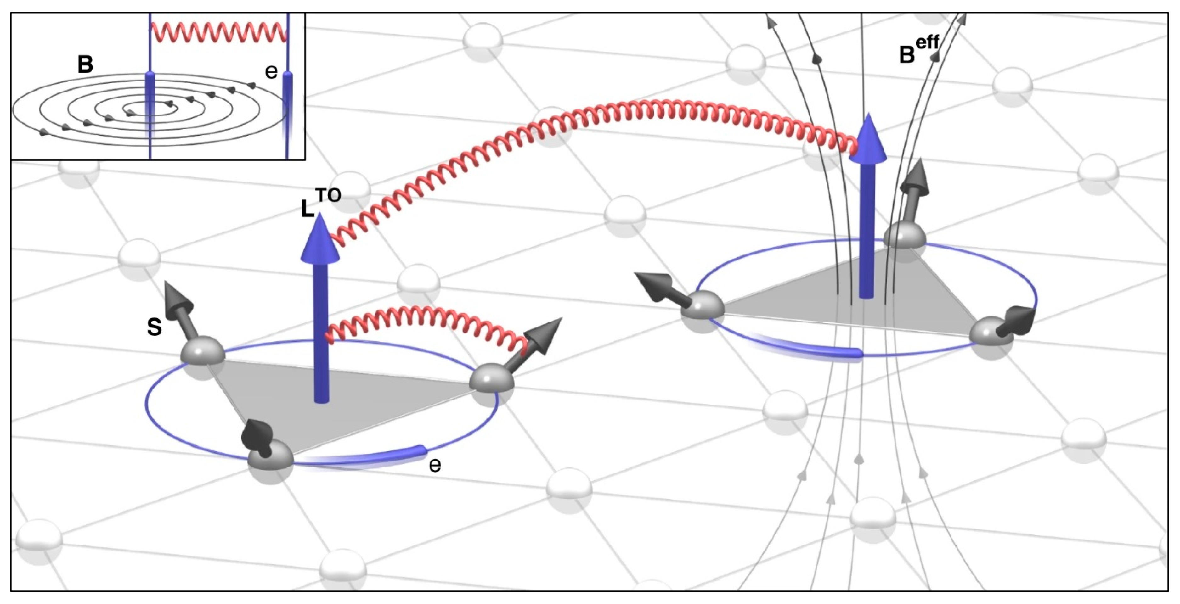
其中单位向量 𝝉𝑖𝑗𝑘∝(𝑹𝑗−𝑹𝑖)×(𝑹𝑘−𝑹𝑖)${\mathit{\tau }}_{ijk}\propto \left({\mathit{R}}_j-{\mathit{R}}_i\right)\times \left({\mathit{R}}_k-{\mathit{R}}_i\right)$ 是沿晶格位 𝑹𝑖${\mathit{R}}_i$ 、 𝑹𝑗${\mathit{R}}_j$ 和 𝑹𝑘${\mathit{R}}_k$ 构成的定向三角形的表面法线。在自旋的三元组中，局部的标量自旋手征性 𝜒𝑖𝑗𝑘=𝑺𝑖⋅(𝑺𝑗×𝑺𝑘)${\chi }_{ijk}={\mathit{S}}_i\cdot \left({\mathit{S}}_j\times {\mathit{S}}_k\right)$ 可以解释为一个虚构的有效磁场 𝑩𝑒ff∝𝜒𝑖𝑗𝑘𝝉𝑖𝑗𝑘${\mathit{B}}^{e\mathrm{ff}}\propto {\chi }_{ijk}{\mathit{\tau }}_{ijk}$ ，这导致由电子在三角形周围跳跃产生的拓扑轨道磁矩（TOM）[129, 130, 131, 132, 133, 134]。拓扑轨道磁矩（TOM）定义为

𝑳𝑇𝑂𝑖=∑(𝑗𝑘)𝑳𝑇𝑂𝑖𝑗𝑘=∑(𝑗𝑘)𝜅𝑇𝑂𝑖𝑗𝑘𝜒𝑖𝑗𝑘𝝉𝑖𝑗𝑘$${\mathit{L}}_i^{TO}={\displaystyle \sum }_{\left(jk\right)}{\mathit{L}}_{ijk}^{TO}={\displaystyle \sum }_{\left(jk\right)}{\kappa }_{ijk}^{TO}{\chi }_{ijk}{\mathit{\tau }}_{ijk}$$

(14)

where 𝜅𝑇𝑂𝑖𝑗𝑘${\kappa }_{ijk}^{TO}$ is the local topological orbital susceptibility. CCI corresponds to the interaction between pairs of topological orbital currents (or TOMs), whose local part can be interpreted as the orbital Zeeman interaction 𝑳𝑇𝑂𝑖⋅𝑩eff${\mathit{L}}_i^{TO}\cdot {\mathit{B}}^{\mathrm{eff}}$. SCI arises from the SOC, which couples the TOM to single spin magnetic moments. An illustration of CCI and SCI is provided in Figure 2. Considerations of CCI and SCI improved the fitting of the total energy in MnGe (see details in Ref. [128]). Moreover, the authors showed the possibility that the CCI may lead to three-dimensional topological spin states and therefore may be vital in deciding the ground state of the spin configurations of MnGe, which was found to be a three-dimensional topological lattice (possibly built up with hedgehogs and anti-hedgehogs) experimentally [135].
局部拓扑轨道磁化率 𝜅𝑇𝑂𝑖𝑗𝑘${\kappa }_{ijk}^{TO}$ 。CCI 对应于拓扑轨道电流对（或 TOMs）之间的相互作用，其局部部分可以解释为轨道塞曼相互作用 𝑳𝑇𝑂𝑖⋅𝑩eff${\mathit{L}}_i^{TO}\cdot {\mathit{B}}^{\mathrm{eff}}$ 。SCI 起源于自旋轨道耦合（SOC），它将 TOM 与单个自旋磁矩耦合。图 2 提供了 CCI 和 SCI 的示意图。考虑 CCI 和 SCI 提高了 MnGe 中总能量的拟合（详见参考文献[128]）。此外，作者展示了 CCI 可能导致三维拓扑自旋状态的可能性，因此可能在决定 MnGe 的自旋配置基态中发挥关键作用，实验上发现 MnGe 是一个三维拓扑晶格（可能由刺猬和反刺猬组成）[135]。

Figure 2. Schematic diagrams of chiral–chiral interactions (CCI) and spin–chiral interactions (SCI), as provided by S. Grytsiuk et al. in Ref. [128]. Spins and topological orbital moments (TOMs) are denoted as black arrows and blue arrows, respectively. CCI can be regarded as interactions between TOMs, while SCI can be interpreted as interactions between TOM and local spins.
图 2. S. Grytsiuk 等人提供的手性-手性相互作用（CCI）和自旋-手性相互作用（SCI）的示意图。自旋和拓扑轨道矩（TOMs）分别用黑色箭头和蓝色箭头表示。CCI 可以被视为 TOMs 之间的相互作用，而 SCI 可以解释为 TOM 和局域自旋之间的相互作用。

A new type of chiral pair interaction 𝑪𝑖𝑗⋅(𝑺𝑖×𝑺𝑗) (𝑺𝑖⋅𝑺𝑗)${\mathit{C}}_{ij}\cdot \left({\mathit{S}}_i\times {\mathit{S}}_j\right) \left({\mathit{S}}_i\cdot {\mathit{S}}_j\right)$, named as chiral biquadratic interaction (CBI), which is the biquadratic equivalent of the DMI, was derived from a microscopic model and demonstrated to be comparable in magnitude to the DMI in magnetic dimers made of 3d elements on Pt(111), Pt(001), Ir(111) and Re(0001) surface with strong SOC [136]. Similar but generalized chiral interactions such as 𝑫𝑖𝑗𝑗𝑘⋅(𝑺𝑗×𝑺𝑘) (𝑺𝑖⋅𝑺𝑗)${\mathit{D}}_{ijjk}\cdot \left({\mathit{S}}_j\times {\mathit{S}}_k\right) \left({\mathit{S}}_i\cdot {\mathit{S}}_j\right)$ and 𝑫𝑖𝑗𝑘𝑙⋅(𝑺𝑘×𝑺𝑙) (𝑺𝑖⋅𝑺𝑗)${\mathit{D}}_{ijkl}\cdot \left({\mathit{S}}_k\times {\mathit{S}}_l\right) \left({\mathit{S}}_i\cdot {\mathit{S}}_j\right)$, named four-spin chiral interactions, were discussed in Ref. [137], and they are found to be important in predicting a correct chirality for a spin spiral state of Fe chains deposited on the Re(0001) surface.
一种新型的手性对相互作用 𝑪𝑖𝑗⋅(𝑺𝑖×𝑺𝑗) (𝑺𝑖⋅𝑺𝑗)${\mathit{C}}_{ij}\cdot \left({\mathit{S}}_i\times {\mathit{S}}_j\right) \left({\mathit{S}}_i\cdot {\mathit{S}}_j\right)$ ，称为手性双二次相互作用（CBI），它是 DMI 的双二次等价形式，从一个微观模型中推导出来，并在 Pt(111)、Pt(001)、Ir(111)和 Re(0001)表面上的 3d 元素磁二聚体中，与 DMI 在强度上相当[136]。类似但更普遍的手性相互作用，如 𝑫𝑖𝑗𝑗𝑘⋅(𝑺𝑗×𝑺𝑘) (𝑺𝑖⋅𝑺𝑗)${\mathit{D}}_{ijjk}\cdot \left({\mathit{S}}_j\times {\mathit{S}}_k\right) \left({\mathit{S}}_i\cdot {\mathit{S}}_j\right)$ 和 𝑫𝑖𝑗𝑘𝑙⋅(𝑺𝑘×𝑺𝑙) (𝑺𝑖⋅𝑺𝑗)${\mathit{D}}_{ijkl}\cdot \left({\mathit{S}}_k\times {\mathit{S}}_l\right) \left({\mathit{S}}_i\cdot {\mathit{S}}_j\right)$ ，称为四自旋手性相互作用，在参考文献[137]中进行了讨论，并发现它们在预测 Re(0001)表面沉积的 Fe 链的螺旋态的正确手性方面非常重要。

When there is a magnetic field, for a nonbipartite lattice, the magnetic field can couple with the spin and produce a new term of the form 𝐽𝑖𝑗𝑘𝑺𝑖⋅(𝑺𝑗×𝑺𝑘)=𝐽𝑖𝑗𝑘𝜒𝑖𝑗𝑘$J_{ijk}{\mathit{S}}_i\cdot \left({\mathit{S}}_j\times {\mathit{S}}_k\right)=J_{ijk}{\chi }_{ijk}$ [138,139], which can be termed the three-spin chiral interaction (TCI) [140]. Such a chiral term can induce a gapless line in frustrated spin-gapped phases, and a critical chiral strength can change the ground state from spiral to Néel quasi-long-range-order phase [138]. This chiral term is also found to produce a chiral spin liquid state [141], where the time-reversal symmetry is broken spontaneously by the emergence of long-range order of scalar chirality [142].
当存在磁场时，对于非二分晶格，磁场可以与自旋耦合，产生形式为 𝐽𝑖𝑗𝑘𝑺𝑖⋅(𝑺𝑗×𝑺𝑘)=𝐽𝑖𝑗𝑘𝜒𝑖𝑗𝑘$J_{ijk}{\mathit{S}}_i\cdot \left({\mathit{S}}_j\times {\mathit{S}}_k\right)=J_{ijk}{\chi }_{ijk}$ [ 138, 139]的新项，这可以称为三自旋手征相互作用（TCI）[ 140]。这样的手征项可以诱导在反铁磁自旋隙相中产生无隙线，一个临界手征强度可以将基态从螺旋相转变为 Néel 准长程有序相[ 138]。这种手征项还发现可以产生手征自旋液体状态[ 141]，其中通过标量手征长程序的出现，自发地破坏了时间反演对称性[ 142]。

2.6. Expansions of Magnetic Interactions
2.6. 磁性相互作用的展开

In general, a complete basis can be used to expand the spin interactions. One example is the spin-cluster expansion (SCE) [143,144,145], where unit vectors denoting the directions of spins are used as independent variables and spherical harmonic functions are used in the expressions of the basis functions. When SOC and the external magnetic field are not important, as mentioned in Section 2.3, only inner products of spins need to be considered. Consequently, the expansion can be
通常，可以使用完备基来展开自旋相互作用。一个例子是自旋簇展开（SCE）[143, 144, 145]，其中使用表示自旋方向的单位向量作为独立变量，并在基函数的表达式中使用球谐函数。当如第 2.3 节所述，自旋轨道耦合（SOC）和外部磁场不重要时，只需要考虑自旋的内积。因此，展开可以

𝐻spin=𝐸0+∑𝑛=1∞𝐽𝑛⎛⎝⎜⎜⎜⎜⎜∑𝑛th nearest pairs 〈𝑘,𝑙〉𝒆𝑘⋅𝒆𝑙⎞⎠⎟⎟⎟⎟⎟+∑𝑛′=1∞𝐽′𝑛′∑𝑛′th type (𝒆𝑘⋅𝒆𝑙)(𝒆𝑚⋅𝒆𝑛)+⋯$$H_{\mathrm{spin}}=E_0+{\displaystyle \sum }_{n=1}^{\infty }{J}_n\left({\displaystyle \sum }_{n\mathrm{th} \mathrm{nearest} \mathrm{pairs} \langle k,l\rangle }{\mathit{e}}_k\cdot {\mathit{e}}_l\right)+{\displaystyle \sum }_{n^{\prime }=1}^{\infty }{J}_{n^{\prime }}^{\prime }{\displaystyle \sum }_{n^{\prime }\mathrm{th} \mathrm{type} }\left({\mathit{e}}_k\cdot {\mathit{e}}_l\right)\left({\mathit{e}}_m\cdot {\mathit{e}}_n\right)+\cdots$$

(15)

as used in Ref. [125]. When using expansions of spin vectors (or directions of the spins), suitable truncations on interaction distances and interaction orders are needed. Otherwise, the number of terms would be infinite, and as a result, the problem would be unsolvable.
在参考文献[125]中所述。当使用自旋矢量的展开（或自旋的方向）时，需要对相互作用距离和相互作用阶数进行适当的截断。否则，项的数量将是无限的，结果问题将无法解决。

3. Methods of Computing the Parameters of Effective Spin Hamiltonian Models
3. 有效自旋哈密顿量模型参数的计算方法

In this part, we mainly discuss the methods of computing the spin interaction parameters based on first-principles calculations of crystals, where periodic boundary conditions are tacitly supposed. These methods include different kinds of energy-mapping analysis (see Section 3.1) and Green’s function method based on magnetic-force linear response theory (see Section 3.2). Discussions on the rigid spin rotation approximation and other assumptions are provided in Section 3.3. The cases of clusters, where periodic boundary conditions do not exist, will be briefly discussed in Section 3.3. Methods of obtaining spin interaction parameters from experiments will also be briefly mentioned in Section 3.3.
在这一部分，我们主要讨论基于晶体第一性原理计算的磁矩相互作用参数的计算方法，其中周期性边界条件被隐含地假设。这些方法包括不同种类的能量映射分析（见第 3.1 节）和基于磁力线性响应理论的格林函数方法（见第 3.2 节）。第 3.3 节提供了关于刚性磁矩旋转近似和其他假设的讨论。第 3.3 节将简要讨论不存在周期性边界条件的簇的情况。第 3.3 节还将简要提及从实验中获得磁矩相互作用参数的方法。

3.1. Energy-Mapping Analysis
3.1. 能量映射分析

In an energy-mapping analysis, we do several first-principles calculations to assess the total energies of different spin configurations. Then, we use the effective spin Hamiltonian to provide the expressions of the total energies of these spin configurations (with the expressions containing several undetermined parameters). By mapping the total energy expressions given by the effective spin Hamiltonian model to the results of first-principles calculations, the values of the undetermined parameters can be estimated. There are several types of energy-mapping analysis. For the first type, a minimal number of configurations are used, and a concrete expression for calculating the parameters can be given in advance. An example is by mapping between the eigenvalues and eigenfunctions of exact Hamiltonians and the effective spin Hamiltonian models (typically the Heisenberg model) to estimate the exchange parameters for relatively simple systems [146,147]. Several broken symmetry (BS) approaches are also of this type, where broken-symmetry states (instead of eigenstates of exact Hamiltonians) are adopted for energy mapping between the models and results of first-principles calculations [147,148]. A typical example of BS approach is the four-state method [148,149] where four special states are chosen for calculating each component of the parameters, which will be introduced in Section 3.1.1. For the second type, more configurations are used, and the parameters in the supposed effective spin Hamiltonian model are determined by employing least-squares fitting, which will be introduced in Section 3.1.2. The third type is similar to the second one, but the concrete form of the effective spin Hamiltonian model is not determined in advance. In the beginning, one includes many terms in the mode Hamiltonians. The relevance of each individual term depends on the fitting performance with respect to first-principles calculations. While selecting the relevant terms for a model Hamiltonian, it is important to search for the minimal Hamiltonian for a given magnetic system, namely, the one with the minimal number of parameters that capture its essential physics. This type of energy-mapping analysis will be introduced in Section 3.1.3.
在能量映射分析中，我们进行了几次基于第一性原理的计算，以评估不同自旋配置的总能量。然后，我们使用有效自旋哈密顿量来提供这些自旋配置的总能量表达式（其中包含几个未确定的参数）。通过将有效自旋哈密顿量模型给出的总能量表达式映射到基于第一性原理的计算结果，可以估计未确定参数的值。存在几种类型的能量映射分析。对于第一种类型，使用最小数量的配置，并且可以预先给出计算参数的具体表达式。一个例子是通过在精确哈密顿量的本征值和本征函数与有效自旋哈密顿量模型（通常是海森堡模型）之间进行映射，以估计相对简单系统的交换参数[ 146, 147]。 几种破缺对称性（BS）方法也属于此类，其中采用破缺对称性状态（而不是精确哈密顿量的本征态）来在模型和第一性原理计算结果之间进行能量映射[147, 148]。BS 方法的典型例子是四种状态方法[148, 149]，其中选择四个特殊状态来计算每个参数分量，这些将在第 3.1.1 节中介绍。对于第二种类型，使用更多的配置，并使用最小二乘法拟合来确定假设的有效自旋哈密顿量模型中的参数，这将在第 3.1.2 节中介绍。第三种类型与第二种类型相似，但事先未确定有效自旋哈密顿量模型的具体形式。最初，在模式哈密顿量中包含许多项。每个单独项的相关性取决于与第一性原理计算的拟合性能。 在为模型哈密顿量选择相关项时，寻找给定磁系统的最小哈密顿量非常重要，即具有最少参数却能捕捉其基本物理的哈密顿量。这种能量映射分析将在第 3.1.3 节中介绍。

In this section, we will mainly focus on the applications in solid state systems with periodic boundary conditions. The total energy of a designated configuration (which is usually a broken-symmetry state) is typically provided by first-principles calculations (e.g., DFT+U calculations) with constrained directions of magnetic moments.
在这一节中，我们将主要关注具有周期性边界条件的固态系统中的应用。指定配置（通常是破缺对称态）的总能量通常由第一性原理计算（例如，DFT+U 计算）提供，其中磁矩的方向受到约束。

3.1.1. Four-State Method  3.1.1. 四态法

The energy-mapping analysis based on four ordered spin states [148,149], also referred to as the four-state method, assumes the effective spin Hamiltonian include only second-order terms (i.e., isotropic Heisenberg terms, DMI terms, Kitaev terms, and SIA terms). Each component of the parameters like 𝐽𝑖𝑗$J_{ij}$, 𝑫𝑖𝑗,𝑥${\mathit{D}}_{ij,x}$, 𝔸𝑖,𝑥𝑦${\mathbb{A}}_{i,xy}$, (𝔸𝑖,𝑦𝑦−𝔸𝑖,𝑥𝑥${\mathbb{A}}_{i,yy}-{\mathbb{A}}_{i,xx}$) and (𝔸𝑖,𝑧𝑧−𝔸𝑖,𝑥𝑥${\mathbb{A}}_{i,zz}-{\mathbb{A}}_{i,xx}$) can be obtained by first-principles calculations for four specified spin states [148]. Taking the isotropic Heisenberg parameter 𝐽𝑖𝑗$J_{ij}$ for example, with the spin-orbit coupling (SOC) switched off during the first-principles calculations, we use 𝐸𝑖𝑗,𝛼𝛽$E_{ij,\alpha \beta }$ (𝛼,𝛽=↑,↓$\alpha ,\beta =\uparrow ,\downarrow$) to denote the energy of the configuration where spin i is parallel or antiparallel to the z direction (if 𝛼=↑or ↓$\alpha =\uparrow \mathrm{or} \downarrow$, respectively), spin j is parallel or antiparallel to the z direction (if 𝛽= ↑or↓$\beta = \uparrow \mathrm{or}\downarrow$, respectively), and all the spins except i and j are kept unchanged in the four states (which will be referred to as the “reference configuration”, usually chosen to be a low-energy collinear state). Then 𝐽𝑖𝑗$J_{ij}$ can be expressed as
基于四种有序自旋状态[148, 149]的能量映射分析，也称为四态方法，假设有效自旋哈密顿量仅包含二阶项（即各向同性海森堡项、各向异性磁化率项、基泰夫项和 SIA 项）。参数的每个分量，如 𝐽𝑖𝑗$J_{ij}$ 、 𝑫𝑖𝑗,𝑥${\mathit{D}}_{ij,x}$ 、 𝔸𝑖,𝑥𝑦${\mathbb{A}}_{i,xy}$ 、( 𝔸𝑖,𝑦𝑦−𝔸𝑖,𝑥𝑥${\mathbb{A}}_{i,yy}-{\mathbb{A}}_{i,xx}$ )和( 𝔸𝑖,𝑧𝑧−𝔸𝑖,𝑥𝑥${\mathbb{A}}_{i,zz}-{\mathbb{A}}_{i,xx}$ )，可以通过对四种指定自旋状态[148]进行第一性原理计算获得。以各向同性海森堡参数 𝐽𝑖𝑗$J_{ij}$ 为例，在第一性原理计算中关闭自旋轨道耦合（SOC）时，我们使用 𝐸𝑖𝑗,𝛼𝛽$E_{ij,\alpha \beta }$ （ 𝛼,𝛽=↑,↓$\alpha ,\beta =\uparrow ,\downarrow$ ）表示自旋平行或反平行于 z 方向（如果 𝛼=↑or ↓$\alpha =\uparrow \mathrm{or} \downarrow$ ，分别），自旋平行或反平行于 z 方向（如果 𝛽= ↑or↓$\beta = \uparrow \mathrm{or}\downarrow$ ，分别），并且除了和之外的所有自旋在四种状态中保持不变（这将被称为“参考配置”，通常选择为低能共线状态）。然后 𝐽𝑖𝑗$J_{ij}$ 可以表示为

𝐽𝑖𝑗=𝐸𝑖𝑗,↑↑+𝐸𝑖𝑗,↓↓−𝐸𝑖𝑗,↑↓−𝐸𝑖𝑗,↓↑4𝑺2$$J_{ij}=\frac{E_{ij,\uparrow \uparrow }+E_{ij,\downarrow \downarrow }-E_{ij,\uparrow \downarrow }-E_{ij,\downarrow \uparrow }}{4{\mathit{S}}^2}$$

(16)

The schematic diagrams of these four states are shown in Figure 3.
这些四种状态的示意图如图 3 所示。

Figure 3. Schematic diagrams of the four states adopted in the four-state method for computing 𝐽𝑖𝑗$J_{ij}$. Except atoms i and j, all the other atoms are omitted in this diagram (which are kept the same in the four states). Spins pointing up and down are indicated with orange and blue balls, respectively. The total energies given by first-principles calculations corresponding to these four states are denoted as (a) 𝐸𝑖𝑗,↑↑$E_{ij,\uparrow \uparrow }$, (b) 𝐸𝑖𝑗,↑↓$E_{ij,\uparrow \downarrow }$, (c) 𝐸𝑖𝑗,↓↑$E_{ij,\downarrow \uparrow }$, and (d) 𝐸𝑖𝑗,↓↓$E_{ij,\downarrow \downarrow }$, respectively.
图 3. 四状态方法计算 𝐽𝑖𝑗$J_{ij}$ 所采用的四种状态的示意图。除原子和，所有其他原子在此图中省略（在四种状态中保持不变）。向上和向下的自旋分别用橙色和蓝色球表示。对应这四种状态的第一性原理计算给出的总能量分别表示为（a） 𝐸𝑖𝑗,↑↑$E_{ij,\uparrow \uparrow }$ ，（b） 𝐸𝑖𝑗,↑↓$E_{ij,\uparrow \downarrow }$ ，（c） 𝐸𝑖𝑗,↓↑$E_{ij,\downarrow \uparrow }$ 和（d） 𝐸𝑖𝑗,↓↓$E_{ij,\downarrow \downarrow }$ 。

In general, the second-order effective spin Hamiltonian takes the form of
通常，二阶有效自旋哈密顿量具有以下形式：

𝐻𝑠pin=∑𝑖,𝑗>𝑖𝑺𝑇𝑖𝕁𝑖𝑗𝑺𝑗+∑𝑖𝑺𝑇𝑖𝔸𝑖𝑺𝑖$$H_{s\mathrm{pin}}={\displaystyle \sum }_{i,j>i}{\mathit{S}}_i^T{\mathbb{J}}_{ij}{\mathit{S}}_j+{\displaystyle \sum }_i{\mathit{S}}_i^T{\mathbb{A}}_i{\mathit{S}}_i$$

(17)

and each component of the matrix 𝕁𝑖𝑗${\mathbb{J}}_{ij}$ and 𝔸𝑖${\mathbb{A}}_i$ can also be obtained by first-principles calculations for four specified spin states. To compute 𝕁𝑖𝑗,𝑎𝑏${\mathbb{J}}_{ij,ab}$ (𝑎,𝑏=𝑥,𝑦,𝑧$a,b=x,y,z$), we use 𝐸𝑖𝑗,𝑎𝑏,𝛼𝛽$E_{ij,ab,\alpha \beta }$ (𝛼,𝛽= ↑,↓$\alpha ,\beta = \uparrow ,\downarrow$) to denote the energy of the configuration where spin i is parallel or antiparallel to the a direction (if 𝛼= ↑or↓$\alpha = \uparrow \mathrm{or}\downarrow$, respectively), spin j is parallel or antiparallel to the b direction (if 𝛽= ↑or↓$\beta = \uparrow \mathrm{or}\downarrow$, respectively), and all the spins except for i and j are kept unchanged and parallel to the c-axis (𝑐=𝑥,𝑦 or 𝑧$c=x,y \mathrm{or} z$, 𝑐≠𝑎$c\ne a$, 𝑐≠𝑏$c\ne b$) with an appropriate reference configuration and kept unchanged. Then, 𝕁𝑖𝑗,𝑎𝑏${\mathbb{J}}_{ij,ab}$ can be expressed as
矩阵 𝕁𝑖𝑗${\mathbb{J}}_{ij}$ 和 𝔸𝑖${\mathbb{A}}_i$ 的每个分量也可以通过针对四个指定的自旋状态进行第一性原理计算而获得。为了计算 𝕁𝑖𝑗,𝑎𝑏${\mathbb{J}}_{ij,ab}$ （ 𝑎,𝑏=𝑥,𝑦,𝑧$a,b=x,y,z$ ），我们使用 𝐸𝑖𝑗,𝑎𝑏,𝛼𝛽$E_{ij,ab,\alpha \beta }$ （ 𝛼,𝛽= ↑,↓$\alpha ,\beta = \uparrow ,\downarrow$ ）表示自旋与 a 方向平行或反平行（如果 𝛼= ↑or↓$\alpha = \uparrow \mathrm{or}\downarrow$ ，分别）的配置能量，自旋与 b 方向平行或反平行（如果 𝛽= ↑or↓$\beta = \uparrow \mathrm{or}\downarrow$ ，分别）的配置能量，并且除了和之外的所有自旋保持不变，并与 c 轴平行（ 𝑐=𝑥,𝑦 or 𝑧$c=x,y \mathrm{or} z$ ， 𝑐≠𝑎$c\ne a$ ， 𝑐≠𝑏$c\ne b$ ）保持不变，并使用适当的参考配置保持不变。然后， 𝕁𝑖𝑗,𝑎𝑏${\mathbb{J}}_{ij,ab}$ 可以表示为

𝕁𝑖𝑗,𝑎𝑏=𝐸𝑖𝑗,𝑎𝑏,↑↑+𝐸𝑖𝑗,𝑎𝑏,↓↓−𝐸𝑖𝑗,𝑎𝑏,↑↓−𝐸𝑖𝑗,𝑎𝑏,↓↑4𝑺2$${\mathbb{J}}_{ij,ab}=\frac{E_{ij,ab,\uparrow \uparrow }+E_{ij,ab,\downarrow \downarrow }-E_{ij,ab,\uparrow \downarrow }-E_{ij,ab,\downarrow \uparrow }}{4{\mathit{S}}^2}$$

(18)

To compute 𝔸𝑖,𝑎𝑏${\mathbb{A}}_{i,ab}$ (𝑎,𝑏=𝑥,𝑦,𝑧$a,b=x,y,z$ with 𝑎≠𝑏$a\ne b$), we use 𝐸𝑖,𝑎𝑏,𝛼𝛽$E_{i,ab,\alpha \beta }$ (𝛼,𝛽= ↑,↓$\alpha ,\beta = \uparrow ,\downarrow$) to denote the energy of the configuration where spin i is parallel to the direction whose a component is ±2√2$\pm \frac{\sqrt{2}}{2}$ (for 𝛼= ↑or↓$\alpha = \uparrow \mathrm{or}\downarrow$, respectively), b component is ±2√2$\pm \frac{\sqrt{2}}{2}$ (for 𝛽= ↑or↓$\beta = \uparrow \mathrm{or}\downarrow$, respectively), and the other component is 0. Here all the spins except for i and j are parallel to the c-axis (𝑐=𝑥,𝑦 or 𝑧$c=x,y \mathrm{or} z$, 𝑐≠𝑎$c\ne a$, 𝑐≠𝑏$c\ne b$) with an appropriate reference configuration. Then, 𝔸𝑖,𝑎𝑏${\mathbb{A}}_{i,ab}$ can be expressed as
为了计算 𝔸𝑖,𝑎𝑏${\mathbb{A}}_{i,ab}$ （ 𝑎,𝑏=𝑥,𝑦,𝑧$a,b=x,y,z$ 与 𝑎≠𝑏$a\ne b$ ），我们使用 𝐸𝑖,𝑎𝑏,𝛼𝛽$E_{i,ab,\alpha \beta }$ （ 𝛼,𝛽= ↑,↓$\alpha ,\beta = \uparrow ,\downarrow$ ）表示自旋平行于方向 a 分量是 ±2√2$\pm \frac{\sqrt{2}}{2}$ （对于 𝛼= ↑or↓$\alpha = \uparrow \mathrm{or}\downarrow$ ，分别），b 分量是 ±2√2$\pm \frac{\sqrt{2}}{2}$ （对于 𝛽= ↑or↓$\beta = \uparrow \mathrm{or}\downarrow$ ，分别），而其他分量是 0 的配置的能量。在这里，除了和之外的所有自旋都与 c 轴（ 𝑐=𝑥,𝑦 or 𝑧$c=x,y \mathrm{or} z$ ， 𝑐≠𝑎$c\ne a$ ， 𝑐≠𝑏$c\ne b$ ）平行，并有一个适当的参考配置。然后， 𝔸𝑖,𝑎𝑏${\mathbb{A}}_{i,ab}$ 可以表示为

𝔸𝑖,𝑎𝑏=𝐸𝑖,𝑎𝑏,↑↑+𝐸𝑖,𝑎𝑏,↓↓−𝐸𝑖,𝑎𝑏,↑↓−𝐸𝑖,𝑎𝑏,↓↑4𝑆2$${\mathbb{A}}_{i,ab}=\frac{E_{i,ab,\uparrow \uparrow }+E_{i,ab,\downarrow \downarrow }-E_{i,ab,\uparrow \downarrow }-E_{i,ab,\downarrow \uparrow }}{4S^2}$$

(19)

To compute (𝔸𝑖,𝑎𝑎−𝔸𝑖,𝑏𝑏)$\left({\mathbb{A}}_{i,aa}-{\mathbb{A}}_{i,bb}\right)$ (𝑎,𝑏=𝑥,𝑦,𝑧$a,b=x,y,z$ with 𝑎≠𝑏$a\ne b$), we use 𝐸𝑖,𝑎𝑏,𝛼𝛽$E_{i,ab,\alpha \beta }$ (𝛼,𝛽= ↑,↓or 0$\alpha ,\beta = \uparrow ,\downarrow \mathrm{or} 0$) to denote the energy of the configuration where spin i is parallel to the direction whose a component is ±1 or 0$\pm 1 \mathrm{or} 0$ (if 𝛼= ↑, ↓or 0$\alpha = \uparrow , \downarrow \mathrm{or} 0$, respectively), b component is ±1 or 0$\pm 1 \mathrm{or} 0$ (if 𝛽= ↑, ↓or 0$\beta = \uparrow , \downarrow \mathrm{or} 0$, respectively) and the other component is 0, while all the spins except i are parallel to the c-axis (𝑐=𝑥,𝑦 or 𝑧$c=x,y \mathrm{or} z$, 𝑐≠𝑎$c\ne a$, 𝑐≠𝑏$c\ne b$) with an appropriate reference configuration. Then (𝔸𝑖,𝑎𝑎−𝔸𝑖,𝑏𝑏)$\left({\mathbb{A}}_{i,aa}-{\mathbb{A}}_{i,bb}\right)$ can be expressed as
为了计算 (𝔸𝑖,𝑎𝑎−𝔸𝑖,𝑏𝑏)$\left({\mathbb{A}}_{i,aa}-{\mathbb{A}}_{i,bb}\right)$ （ 𝑎,𝑏=𝑥,𝑦,𝑧$a,b=x,y,z$ 与 𝑎≠𝑏$a\ne b$ ），我们使用 𝐸𝑖,𝑎𝑏,𝛼𝛽$E_{i,ab,\alpha \beta }$ （ 𝛼,𝛽= ↑,↓or 0$\alpha ,\beta = \uparrow ,\downarrow \mathrm{or} 0$ ）表示自旋平行于方向 a 分量是 ±1 or 0$\pm 1 \mathrm{or} 0$ （如果 𝛼= ↑, ↓or 0$\alpha = \uparrow , \downarrow \mathrm{or} 0$ ，分别），b 分量是 ±1 or 0$\pm 1 \mathrm{or} 0$ （如果 𝛽= ↑, ↓or 0$\beta = \uparrow , \downarrow \mathrm{or} 0$ ，分别）而其他分量是 0 的配置能量，而除了自旋外的所有自旋都平行于 c 轴（ 𝑐=𝑥,𝑦 or 𝑧$c=x,y \mathrm{or} z$ ， 𝑐≠𝑎$c\ne a$ ， 𝑐≠𝑏$c\ne b$ ）并使用适当的参考配置。然后 (𝔸𝑖,𝑎𝑎−𝔸𝑖,𝑏𝑏)$\left({\mathbb{A}}_{i,aa}-{\mathbb{A}}_{i,bb}\right)$ 可以表示为

𝔸𝑖,𝑎𝑎−𝔸𝑖,𝑏𝑏=𝐸𝑖,𝑎𝑏,↑0+𝐸𝑖,𝑎𝑏,↓0−𝐸𝑖,𝑎𝑏,0↑−𝐸𝑖,𝑎𝑏,0↓4𝑆2$${\mathbb{A}}_{i,aa}-{\mathbb{A}}_{i,bb}=\frac{E_{i,ab,\uparrow 0}+E_{i,ab,\downarrow 0}-E_{i,ab,0\uparrow }-E_{i,ab,0\downarrow }}{4S^2}$$

(20)

It is easy to verify that, by employing this four-state method, each component of the 𝕁𝑖𝑗${\mathbb{J}}_{ij}$ and 𝔸𝑖${\mathbb{A}}_i$ can be obtained with the effects of other second-order terms entirely cancelled. Now we take the effects of fourth-order terms (without SOC) into account and check if the algorithms for computing 𝕁𝑖𝑗${\mathbb{J}}_{ij}$ and 𝔸𝑖${\mathbb{A}}_i$ are still rigorous. For 𝔸𝑖${\mathbb{A}}_i$, we can find out that the effects of all these terms are correctly cancelled. For 𝕁𝑖𝑗${\mathbb{J}}_{ij}$, the effects of biquadratic terms, three-body fourth-order terms, and most of the four-spin ring coupling terms are perfectly cancelled, while only the terms like (𝑺𝑖⋅𝑺𝑗)(𝑺𝑘⋅𝑺𝑙)$\left({\mathit{S}}_i\cdot {\mathit{S}}_j\right)\left({\mathit{S}}_k\cdot {\mathit{S}}_l\right)$ (𝑘,𝑙≠𝑖,𝑗$k,l\ne i,j$) will interfere with the calculation of 𝐽𝑖𝑗$J_{ij}$ because (𝑺𝑘⋅𝑺𝑙)$\left({\mathit{S}}_k\cdot {\mathit{S}}_l\right)$ is constant during the calculation and therefore mixed with the contribution of 𝐽𝑖𝑗(𝑺𝑖⋅𝑺𝑗)$J_{ij}\left({\mathit{S}}_i\cdot {\mathit{S}}_j\right)$. The error of the calculated 𝐽𝑖𝑗$J_{ij}$ originated from four-spin ring coupling terms
通过采用这种方法，很容易验证，通过使用这种方法，可以完全消除其他二阶项的影响，从而获得 𝕁𝑖𝑗${\mathbb{J}}_{ij}$ 和 𝔸𝑖${\mathbb{A}}_i$ 的每个分量。现在我们考虑四阶项的影响（不考虑 SOC），并检查计算 𝕁𝑖𝑗${\mathbb{J}}_{ij}$ 和 𝔸𝑖${\mathbb{A}}_i$ 的算法是否仍然严格。对于 𝔸𝑖${\mathbb{A}}_i$ ，我们可以发现所有这些项的影响都得到了正确的消除。对于 𝕁𝑖𝑗${\mathbb{J}}_{ij}$ ，双曲项、三体四阶项和大多数四自旋环耦合项的影响得到了完美的消除，而只有像 (𝑺𝑖⋅𝑺𝑗)(𝑺𝑘⋅𝑺𝑙)$\left({\mathit{S}}_i\cdot {\mathit{S}}_j\right)\left({\mathit{S}}_k\cdot {\mathit{S}}_l\right)$ （ 𝑘,𝑙≠𝑖,𝑗$k,l\ne i,j$ ）这样的项会干扰 𝐽𝑖𝑗$J_{ij}$ 的计算，因为 (𝑺𝑘⋅𝑺𝑙)$\left({\mathit{S}}_k\cdot {\mathit{S}}_l\right)$ 在计算过程中是常数，因此与 𝐽𝑖𝑗(𝑺𝑖⋅𝑺𝑗)$J_{ij}\left({\mathit{S}}_i\cdot {\mathit{S}}_j\right)$ 的贡献混合在一起。计算出的 𝐽𝑖𝑗$J_{ij}$ 误差源于四自旋环耦合项

∑𝑖,𝑗>𝑖,𝑘>𝑖,𝑙>𝑘𝐾𝑖𝑗𝑘𝑙(𝑺𝑖⋅𝑺𝑗)(𝑺𝑘⋅𝑺𝑙)$${\displaystyle \sum }_{\begin{array}{c}i,j>i,\\ k>i,\\ l>k\end{array}}{K}_{ijkl}\left({\mathit{S}}_i\cdot {\mathit{S}}_j\right)\left({\mathit{S}}_k\cdot {\mathit{S}}_l\right)$$

(21)

is given by
由...给出

∑𝑘≠𝑖 𝑜𝑟 𝑗𝑙≠𝑖 𝑜𝑟 𝑗(𝑙>𝑘)𝐾𝑖𝑗𝑘𝑙(𝑺𝑘⋅𝑺𝑙)$${\displaystyle \sum }_{\begin{array}{c}k\ne i or j\\ l\ne i or j\\ (l>k)\end{array}}{K}_{ijkl}\left({\mathit{S}}_k\cdot {\mathit{S}}_l\right)$$

(22)

while there is no easy way to get rid of this problem perfectly. Other parts of the 𝕁𝑖𝑗${\mathbb{J}}_{ij}$ (including 𝔻𝑖𝑗${\mathbb{D}}_{ij}$ and 𝕂𝑖𝑗${\mathbb{K}}_{ij}$) are not affected by these fourth-order terms (without SOC), but by other types of fourth-order terms (like four-spin chiral interactions) if SOC is taken into account (because of the similar reason).
在磁体中旋转哈密顿量：理论计算 当没有简单的方法完美解决这个问题。 𝕁𝑖𝑗${\mathbb{J}}_{ij}$ 的其他部分（包括 𝔻𝑖𝑗${\mathbb{D}}_{ij}$ 和 𝕂𝑖𝑗${\mathbb{K}}_{ij}$ ）在没有自旋轨道耦合（SOC）的情况下不受这些四阶项的影响，但如果考虑自旋轨道耦合（由于类似的原因），则受其他类型的四阶项（如四自旋手征相互作用）的影响。

In Ref. [122], the four-spin ring coupling interaction is found to be important in TbMnO₃, and therefore leads to instability in calculating the Heisenberg parameters using the four-state method when changing the reference configurations. This problem is remedied by calculating the Heisenberg parameter 𝐽𝑖𝑗$J_{ij}$ twice with the four-state method using the FM and A-type AFM (A-AFM, see Figure 4c) as the reference configurations, and use their average value as the final estimation of 𝐽𝑖𝑗$J_{ij}$. The parameter of the vital ring coupling interaction is obtained by calculating the difference between the two calculated 𝐽𝑖𝑗$J_{ij}$ values (with FM and A-AFM reference configurations, respectively). This effective remedy is based on the assumption that only one kind of ring coupling interaction is essential. However, if there are more kinds of significant ring coupling or if we do not know which ring coupling is essential in advance, such a method of calculating 𝐽𝑖𝑗$J_{ij}$ is still not very trustworthy. Nevertheless, it is found that by taking the average of the calculated 𝐽𝑖𝑗$J_{ij}$ with four-state method with FM and G-type AFM (G-AFM, see Figure 4a) reference configurations, the influences of 𝐾𝑖𝑗𝑘𝑙(𝑺𝑖⋅𝑺𝑗)(𝑺𝑘⋅𝑺𝑙)$K_{ijkl}\left({\mathit{S}}_i\cdot {\mathit{S}}_j\right)\left({\mathit{S}}_k\cdot {\mathit{S}}_l\right)$ with k and l being nearest pairs are eliminated. The terms 𝐾𝑖𝑗𝑘𝑙(𝑺𝑖⋅𝑺𝑗)(𝑺𝑘⋅𝑺𝑙)$K_{ijkl}\left({\mathit{S}}_i\cdot {\mathit{S}}_j\right)\left({\mathit{S}}_k\cdot {\mathit{S}}_l\right)$ with non-nearest pairs of k and l still interfere with the calculation of 𝐽𝑖𝑗$J_{ij}$, but they are generally very weak. Therefore, such a remedy to calculate 𝐽𝑖𝑗$J_{ij}$ using the four-state method should work well in most cases. In cases when a G-AFM state (in which all the nearest pairs of spins are antiparallelly aligned) cannot be defined (e.g., a triangular or a Kagomé lattice), there may be more than two reference configurations to use in the four-state method so as to eliminate the effects of 𝐾𝑖𝑗𝑘𝑙(𝑺𝑖⋅𝑺𝑗)(𝑺𝑘⋅𝑺𝑙)$K_{ijkl}\left({\mathit{S}}_i\cdot {\mathit{S}}_j\right)\left({\mathit{S}}_k\cdot {\mathit{S}}_l\right)$ terms with non-nearest pairs of k and l. These reference configurations need to be designed carefully according to the specific circumstances to get rid of the effects of 𝐾𝑖𝑗𝑘𝑙(𝑺𝑖⋅𝑺𝑗)(𝑺𝑘⋅𝑺𝑙)$K_{ijkl}\left({\mathit{S}}_i\cdot {\mathit{S}}_j\right)\left({\mathit{S}}_k\cdot {\mathit{S}}_l\right)$ terms as much as possible.
在参考文献[122]中，发现四自旋环耦合相互作用在 TbMnO ₃ 中很重要，因此当改变参考配置时，使用四态法计算海森堡参数会导致不稳定性。这个问题通过使用 FM 和 A 型反铁磁（A-AFM，见图 4c）作为参考配置，用四态法计算海森堡参数 𝐽𝑖𝑗$J_{ij}$ 两次，并使用它们的平均值作为 𝐽𝑖𝑗$J_{ij}$ 的最终估计值来修复。通过计算两种计算得到的 𝐽𝑖𝑗$J_{ij}$ 值（分别使用 FM 和 A-AFM 参考配置）之间的差异，获得了关键环耦合相互作用的参数。这种有效的修复基于假设只有一种环耦合相互作用是关键的。然而，如果有更多种类的显著环耦合，或者我们事先不知道哪种环耦合是关键的，这种计算 𝐽𝑖𝑗$J_{ij}$ 的方法仍然不太可靠。 尽管如此，研究发现，通过取使用 FM 和 G 型 AFM（G-AFM，见图 4a）参考配置的四状态方法计算的 𝐽𝑖𝑗$J_{ij}$ 的平均值，消除了 𝐾𝑖𝑗𝑘𝑙(𝑺𝑖⋅𝑺𝑗)(𝑺𝑘⋅𝑺𝑙)$K_{ijkl}\left({\mathit{S}}_i\cdot {\mathit{S}}_j\right)\left({\mathit{S}}_k\cdot {\mathit{S}}_l\right)$ 中 k 和为最近邻对的影响。 𝐾𝑖𝑗𝑘𝑙(𝑺𝑖⋅𝑺𝑗)(𝑺𝑘⋅𝑺𝑙)$K_{ijkl}\left({\mathit{S}}_i\cdot {\mathit{S}}_j\right)\left({\mathit{S}}_k\cdot {\mathit{S}}_l\right)$ 中非最近邻对的 k 和项仍然会干扰 𝐽𝑖𝑗$J_{ij}$ 的计算，但它们通常非常微弱。因此，使用四状态方法计算 𝐽𝑖𝑗$J_{ij}$ 的这种补救措施在大多数情况下应该有效。在无法定义 G-AFM 状态（其中所有最近邻自旋对都是反平行排列）的情况下（例如，三角形或 Kagomé晶格），在四状态方法中可能需要使用超过两个参考配置，以消除 𝐾𝑖𝑗𝑘𝑙(𝑺𝑖⋅𝑺𝑗)(𝑺𝑘⋅𝑺𝑙)$K_{ijkl}\left({\mathit{S}}_i\cdot {\mathit{S}}_j\right)\left({\mathit{S}}_k\cdot {\mathit{S}}_l\right)$ 项中非最近邻对的 k 和的影响。这些参考配置需要根据具体情况仔细设计，以尽可能消除 𝐾𝑖𝑗𝑘𝑙(𝑺𝑖⋅𝑺𝑗)(𝑺𝑘⋅𝑺𝑙)$K_{ijkl}\left({\mathit{S}}_i\cdot {\mathit{S}}_j\right)\left({\mathit{S}}_k\cdot {\mathit{S}}_l\right)$ 项的影响。

Figure 4. Schematic diagrams of (a) G-type AFM, (b) C-type AFM, and (c) C-type AFM states. Spins pointing to two opposite directions (e.g., up and down) are indicated with orange and blue balls, respectively.
图 4. (a) G 型自旋晶格，(b) C 型自旋晶格，和(c) C 型自旋晶格状态示意图。分别用橙色和蓝色球表示指向两个相反方向（例如，向上和向下）的磁矩。

The main advantages of the four-state method are its relatively small amount of first-principles calculations and its relatively good cancellations of other relevant terms. A weakness is that it cannot analyze the uncertainties of the parameters, so that we do not know how precise those estimated values are. Another weakness, which is also shared with other energy-mapping analysis methods, is that the computed 𝕁𝑖𝑗${\mathbb{J}}_{ij}$ between 𝑺𝑖${\mathit{S}}_i$ and 𝑺𝑗${\mathit{S}}_j$ is actually the sum over 𝕁𝑖𝑗′${\mathbb{J}}_{i{j}^{\prime }}$ with any lattice vector 𝑹=𝒓𝑗′−𝒓𝑗$\mathit{R}={\mathit{r}}_{j^{\prime }}-{\mathit{r}}_j$. Therefore, to get rid of the effects of other spin pairs, a relatively large supercell is needed.
四态方法的主要优点是其相对较少的基于第一性原理的计算量以及相对较好的其他相关项的抵消。一个弱点是它不能分析参数的不确定性，因此我们不知道那些估计值有多精确。另一个弱点，这也是与其他能量映射分析方法共有的，即计算出的 𝕁𝑖𝑗${\mathbb{J}}_{ij}$ 实际上是 𝑺𝑖${\mathit{S}}_i$ 和 𝑺𝑗${\mathit{S}}_j$ 之间的 𝕁𝑖𝑗′${\mathbb{J}}_{i{j}^{\prime }}$ 的任何晶格向量 𝑹=𝒓𝑗′−𝒓𝑗$\mathit{R}={\mathit{r}}_{j^{\prime }}-{\mathit{r}}_j$ 的总和。因此，为了消除其他自旋对的影响，需要相对较大的超胞。

The four-state method can also be generalized to compute biquadratic parameters, where the SOC needs to be switched off during the first-principles calculations. For calculating 𝐾𝑖𝑗$K_{ij}$ in the term 𝐾𝑖𝑗(𝑺𝑖⋅𝑺𝑗)2$K_{ij}{\left({\mathit{S}}_i\cdot {\mathit{S}}_j\right)}^2$, we can let 𝑺𝑖${\mathit{S}}_i$ pointing to the (1,0,0)$\left(1,0,0\right)$ direction, 𝑺𝑗${\mathit{S}}_j$ pointing to the (1,0,0)$\left(1,0,0\right)$, (−1,0,0)$\left(-1,0,0\right)$, (12√,12√,0)$\left(\frac{1}{\sqrt{2}},\frac{1}{\sqrt{2}},0\right)$ and (−12√,−12√,0)$\left(-\frac{1}{\sqrt{2}},-\frac{1}{\sqrt{2}},0\right)$ directions, with other spins parallel to the z-axis. The corresponding total energies are denoted as 𝐸1$E_1$, 𝐸2$E_2$, 𝐸3$E_3$, and 𝐸4$E_4$, respectively. Then the 𝐾𝑖𝑗$K_{ij}$ can be expressed as
四态方法也可以推广到计算双二次参数，其中在第一性原理计算中需要关闭自旋轨道耦合（SOC）。对于计算项 𝐾𝑖𝑗(𝑺𝑖⋅𝑺𝑗)2$K_{ij}{\left({\mathit{S}}_i\cdot {\mathit{S}}_j\right)}^2$ 中的 𝐾𝑖𝑗$K_{ij}$ ，我们可以让 𝑺𝑖${\mathit{S}}_i$ 指向 (1,0,0)$\left(1,0,0\right)$ 方向， 𝑺𝑗${\mathit{S}}_j$ 指向 (1,0,0)$\left(1,0,0\right)$ 、 (−1,0,0)$\left(-1,0,0\right)$ 、 (12√,12√,0)$\left(\frac{1}{\sqrt{2}},\frac{1}{\sqrt{2}},0\right)$ 和 (−12√,−12√,0)$\left(-\frac{1}{\sqrt{2}},-\frac{1}{\sqrt{2}},0\right)$ 方向，其他自旋与 z 轴平行。相应的总能量分别表示为 𝐸1$E_1$ 、 𝐸2$E_2$ 、 𝐸3$E_3$ 和 𝐸4$E_4$ 。然后 𝐾𝑖𝑗$K_{ij}$ 可以表示为

𝐾𝑖𝑗=𝐸1+𝐸2−𝐸3−𝐸4$$K_{ij}=E_1+E_2-E_3-E_4$$

(23)

It can be easily checked that the effects of other terms not higher than fourth order are totally eliminated. Therefore, this approach of calculating 𝐾𝑖𝑗$K_{ij}$ should be relatively rigorous theoretically.
可以很容易地验证，高于四阶的其他项的影响被完全消除。因此，这种计算 𝐾𝑖𝑗$K_{ij}$ 的方法在理论上应该是相对严格的。

Note that the four-state methods [148,149] could also give the derivatives of exchange interactions with respect to the atomic displacements without doing additional first-principles calculations due to the Hellmann-Feynman theorem. These derivatives are useful for the study of spin-lattice coupling related phenomena.
请注意，四种状态的方法[148, 149]也可以在不进行额外的第一性原理计算的情况下，由于 Hellmann-Feynman 定理，给出交换相互作用相对于原子位移的导数。这些导数对于研究自旋-晶格耦合相关现象是有用的。

3.1.2. Direct Least Squares Fitting
3.1.2. 直接最小二乘拟合

Another type of energy-mapping analysis, instead of the four-state method, uses more first-principles calculations with different spin configurations and fits the results to the effective spin Hamiltonian using the least-squares method to estimate the parameters [74,122,123,124]. Ways of choosing spin configurations can depend on which parameters to estimate.
另一种能量映射分析，不是使用四态方法，而是使用更多基于第一性原理的计算，采用不同的自旋配置，并使用最小二乘法将结果拟合到有效自旋哈密顿量，以估计参数[74, 122, 123, 124]。选择自旋配置的方法取决于要估计的参数。

In Ref. [74], for the four Mn sites in a unit cell of YMnO₃, the polar and azimuthal angles (𝜃,φ)$\left(\theta ,\mathsf{\phi }\right)$ of their spins are given by (0, 0)$\left(0, 0\right)$, (0, 0)$\left(0, 0\right)$, (𝜃, 3𝜋2)$\left(\theta , \frac{3\pi }{2}\right)$, and (𝜃, 𝜋2)$\left(\theta , \frac{\pi }{2}\right)$, respectively. By changing the 𝜃$\theta$ from 0°$°$ to 180°$°$, different configurations are produced. If the effective spin Hamiltonian only contains Heisenberg terms, there will be a systematic deviation between the predicted value given by the effective Hamiltonian and the calculated value given by first-principles calculations. Such a deviation is well remedied by adding biquadratic exchange interactions into the effective Hamiltonian model. Thus, the biquadratic parameters can be fitted. Similar approaches were adopted by others to calculate and show the importance of biquadratic parameters and topological chiral–chiral contributions [122,123,124,128]. Apart from using an angular variable for generating spin configurations, using two or more variables is also practicable, or randomly chosen directions [106] can also be considered. Thus, more diverse configurations will be produced. The least-squares fitting will also work, but whether a systematic deviation exists will not be as apparent as the case when only one angular variable is used for generating configurations, and the fitting task may be more laborious.
在参考文献[74]中，对于 YMnO ₃ 的一个晶胞中的四个 Mn 位点，它们的自旋的极角和方位角 (𝜃,φ)$\left(\theta ,\mathsf{\phi }\right)$ 分别由 (0, 0)$\left(0, 0\right)$ 、 (0, 0)$\left(0, 0\right)$ 、 (𝜃, 3𝜋2)$\left(\theta , \frac{3\pi }{2}\right)$ 和 (𝜃, 𝜋2)$\left(\theta , \frac{\pi }{2}\right)$ 给出。通过将 𝜃$\theta$ 从 0 °$°$ 变为 180 °$°$ ，可以得到不同的配置。如果有效自旋哈密顿量只包含海森堡项，那么有效哈密顿量给出的预测值和第一性原理计算给出的计算值之间将存在系统偏差。这种偏差可以通过将双二次交换相互作用添加到有效哈密顿量模型中得到有效纠正。因此，可以拟合双二次参数。其他人也采用了类似的方法来计算和展示双二次参数和拓扑手性-手性贡献的重要性[122, 123, 124, 128]。除了使用角度变量来生成自旋配置外，使用两个或更多变量也是可行的，或者也可以考虑随机选择的方向[106]。因此，将产生更多样化的配置。 最小二乘拟合也会有效，但是否存在系统性偏差可能不如仅使用一个角变量生成配置时那么明显，拟合任务可能更加费力。

The main virtues of this method are that the reliability of the model can be checked by the fitting performance and that the uncertainties of the parameters can be estimated if needed. This method is especially suitable for calculations of biquadratic parameters and topological CCI. However, when talking about calculations of Heisenberg parameters, this method needs more first-principles calculations and is thus less efficient. Furthermore, the fitted result of the Heisenberg parameter 𝐽𝑖𝑗$J_{ij}$ is vulnerable to the effects of other fourth-order interactions such as terms as (𝑺𝑖⋅𝑺𝑗)(𝑺𝑖⋅𝑺𝑘)$\left({\mathit{S}}_i\cdot {\mathit{S}}_j\right)\left({\mathit{S}}_i\cdot {\mathit{S}}_k\right)$ and (𝑺𝑖⋅𝑺𝑗)(𝑺𝑘⋅𝑺𝑙)$\left({\mathit{S}}_i\cdot {\mathit{S}}_j\right)\left({\mathit{S}}_k\cdot {\mathit{S}}_l\right)$. Therefore, the estimations of the Heisenberg parameters may not be very reliable if any of such fourth-order interactions are essential. This problem can be remedied by adding the related terms into the effective Hamiltonian model, while it is not easy to decide which terms to include in the model beforehand.
该方法的主要优点是可以通过拟合性能来检查模型的可靠性，并在需要时估计参数的不确定性。此方法特别适用于双二次参数和拓扑 CCI 的计算。然而，当谈到海森堡参数的计算时，此方法需要更多的第一性原理计算，因此效率较低。此外，海森堡参数 𝐽𝑖𝑗$J_{ij}$ 的拟合结果容易受到其他四阶相互作用（如 (𝑺𝑖⋅𝑺𝑗)(𝑺𝑖⋅𝑺𝑘)$\left({\mathit{S}}_i\cdot {\mathit{S}}_j\right)\left({\mathit{S}}_i\cdot {\mathit{S}}_k\right)$ 和 (𝑺𝑖⋅𝑺𝑗)(𝑺𝑘⋅𝑺𝑙)$\left({\mathit{S}}_i\cdot {\mathit{S}}_j\right)\left({\mathit{S}}_k\cdot {\mathit{S}}_l\right)$ 等项）的影响。因此，如果这些四阶相互作用是基本的，那么海森堡参数的估计可能不太可靠。可以通过将相关项添加到有效哈密顿模型中解决这个问题，但在事先决定要包含哪些项在模型中并不容易。

A possible way to get rid of the effects of other high-order terms is to perform artificial calculations where most of the magnetic ions are replaced by similar but nonmagnetic ions (e.g., substituting Fe³⁺ ions with nonmagnetic Al³⁺ ions) except for one or more ions to be studied [150]. For example, when calculating SIA, only one magnetic ion is not substituted, and by rotating this magnetic ion and calculating the total energy, the SIA can be studied. When studying two-body interactions between 𝑺𝑖${\mathit{S}}_i$ and 𝑺𝑗${\mathit{S}}_j$, only two magnetic ions (at site i and j) are not substituted, and by rotating the spins (or magnetic moments) of these two magnetic ions, the interactions between them can be studied. Such a technique of substituting atoms can be applied to energy mapping analysis based on either the four-state method or least-squares fitting. In this way, effects from interactions involving other sites are effectively avoided. Nevertheless, this substitution method can make the chemical environments of the remaining magnetic ions different from those in the system with no substitution. This may make the calculations of the interaction parameters untrustworthy.
一种消除其他高阶项影响的方法是在人工计算中用类似但非磁性的离子替换大部分磁性离子（例如，用非磁性的 Al ³⁺ 离子替换 Fe ³⁺ 离子），除了一个或多个要研究的离子[150]。例如，在计算 SIA 时，只有一个磁性离子没有被替换，通过旋转这个磁性离子并计算总能量，可以研究 SIA。当研究 𝑺𝑖${\mathit{S}}_i$ 和 𝑺𝑗${\mathit{S}}_j$ 之间的双体相互作用时，只有两个磁性离子（在位置和）没有被替换，通过旋转这两个磁性离子的自旋（或磁矩），可以研究它们之间的相互作用。这种替换原子的技术可以应用于基于四态法或最小二乘拟合的能量映射分析。这样，涉及其他位置相互作用的效应就可以有效地避免。然而，这种替换方法可能会使剩余磁性离子的化学环境与没有替换的系统中的化学环境不同。这可能会使相互作用参数的计算不可靠。

3.1.3. Methods Based on Expansions and Selecting Important Terms
3.1.3. 基于展开和选择重要项的方法

The traditional energy-mapping analysis needs to construct an effective spin Hamiltonian first and then fit the undetermined parameters. However, it is not easy to give a perfect guess, especially when high-order interactions are essential. Such problems can be solved by considering almost all the possible terms utilizing some particular expansion with appropriate truncations. Usually, there are too many possible terms to be considered, so a direct fitting is impracticable; it requires at least as many first-principles calculations as the number of terms to determine, but leads to over-fitting problems due to too many parameters to determine. So, it is necessary to decide whether or not to include each term into the effective spin Hamiltonian on the basis of their contributions to the fitting performance.
传统的能量映射分析需要首先构建一个有效的自旋哈密顿量，然后拟合未确定的参数。然而，给出一个完美的猜测并不容易，尤其是在高阶相互作用至关重要时。这些问题可以通过考虑几乎所有可能的项，利用一些特定的展开和适当的截断来解决。通常，要考虑的可能项太多，所以直接拟合是不切实际的；它至少需要与确定项数相同数量的第一性原理计算，但由于参数太多而可能导致过拟合问题。因此，有必要根据它们对拟合性能的贡献来决定是否将每个项包含在有效自旋哈密顿量中。

In Ref. [145], SCE is adopted for the expansion of spin interactions of bcc and fcc Fe. After truncations based on the interacting distance and interaction orders, they considered 154 (179) possible different interaction terms in bcc (fcc) Fe. They randomly generated 3954 (835) different spin configurations in a 2 × 2 × 2 supercell for fitting. Their method of choosing terms is as follows: starting from the effective Hamiltonian model with only a constant term, try adding each possible term into the temporary model and accept the one providing the best fitting performance, in which way the terms are added to the model one by one. This method is the forward selection in variable selection problems, which is simple and straightforward, and it works well in most cases. However, this method may include unnecessary interactions to the effect Hamiltonian.
在参考文献[145]中，采用 SCE 方法对体心立方和面心立方 Fe 的磁矩相互作用进行展开。基于相互作用距离和相互作用阶数进行截断后，他们考虑了体心立方（面心立方）Fe 中 154（179）个可能的不同相互作用项。他们在 2×2×2 超胞中随机生成了 3954（835）个不同的磁矩配置以进行拟合。他们选择项的方法如下：从仅包含常数项的有效哈密顿量模型开始，尝试将每个可能的项添加到临时模型中，并接受提供最佳拟合性能的那个项，这样一项一项地将项添加到模型中。这种方法是变量选择问题中的正向选择，简单直接，在大多数情况下效果良好。然而，这种方法可能会将不必要的相互作用引入到有效哈密顿量中。

In Ref. [125], a machine learning method for constructing Hamiltonian (MLMCH) is proposed, which is more efficient and more reliable than the traditional forward selection method. Firstly, a testing set is used to avoid over-fitting problems. Secondly, not only adding terms but also deleting and substituting terms are considered during the search for the appropriate model. Thus, if an added term is judged to be unnecessary, it can still be removed from the model afterward. A penalty factor 𝑝𝜆$p^{\mathit{\lambda }}$ (𝜆≥1$\lambda \ge 1$), where 𝑝$p$ is the number of parameters in the temporary model and 𝜆$\lambda$ is a given parameter, is used together with the loss function 𝜎2${\sigma }^2$ (the fitting variance) to select models with fewer parameters. Several techniques are used to reduce the search space and enhance the search efficiency to select important terms out of tens of thousands of possible terms. The flow charts of this method of variable selection as well as the forward selection method are shown in Figure 5.
在参考文献[125]中，提出了一种构建哈密顿量（MLMCH）的机器学习方法，该方法比传统的正向选择方法更高效、更可靠。首先，使用测试集来避免过拟合问题。其次，在寻找合适的模型时，不仅考虑添加项，还考虑删除和替换项。因此，如果判断添加的项是不必要的，之后仍可以从模型中移除。使用惩罚因子 𝑝𝜆$p^{\mathit{\lambda }}$ （ 𝜆≥1$\lambda \ge 1$ ），其中 𝑝$p$ 是临时模型中的参数数量， 𝜆$\lambda$ 是给定的参数，与损失函数 𝜎2${\sigma }^2$ （拟合方差）一起使用，以选择参数更少的模型。使用几种技术来减少搜索空间并提高搜索效率，以从成千上万的可能项中选择重要的项。该变量选择方法的流程图以及正向选择方法的流程图如图 5 所示。

Figure 5. Flow charts of several methods of variable selection. In these flow charts, the fitting variance 𝜎2${\sigma }^2$ estimated by the training set and the testing set are denoted as 𝜎2̂$\widehat{{\sigma }^2}$ and 𝜎′2̂$\widehat{{{\sigma }^{\prime }}^2}$, respectively. (a) The traditional forward selection method as adopted in Ref. [145]. (b) The forward selection method using a testing set to check if over-fitting problems occur. (c) A simplified flow chart of the algorithm used in MLMCH [125], where some details are omitted. A testing set is used to check if over-fitting problems occur. The criterion for a better model is a smaller (𝜎2̂⋅𝜆𝑝)$\left(\widehat{{\sigma }^2}\cdot {\lambda }^p\right)$ with 𝜆≥1$\lambda \ge 1$. There are 𝑁𝜆$N_{\lambda }$ values of 𝜆$\lambda$, which are set in advance, saved in the array “lambdas(1: 𝑁𝜆$N_{\lambda }$)”, whose components are usually arranged in descending order of magnitude. For each value of 𝜆$\lambda$, the best model is selected by using the criterion (𝜎2̂⋅𝜆𝑝)$\left(\widehat{{\sigma }^2}\cdot {\lambda }^p\right)$.
图 5. 几种变量选择方法的流程图。在这些流程图中，由训练集和测试集估计的拟合方差分别表示为 𝜎2̂$\widehat{{\sigma }^2}$ 和 𝜎′2̂$\widehat{{{\sigma }^{\prime }}^2}$ 。(a)采用参考文献[145]的传统正向选择方法。(b)使用测试集检查是否出现过拟合问题的正向选择方法。(c)MLMCH [125]中使用的算法的简化流程图，其中省略了一些细节。使用测试集检查是否出现过拟合问题。更好模型的判据是更小的 (𝜎2̂⋅𝜆𝑝)$\left(\widehat{{\sigma }^2}\cdot {\lambda }^p\right)$ ，其中 𝜆≥1$\lambda \ge 1$ 。有 𝑁𝜆$N_{\lambda }$ 个 𝜆$\lambda$ 的值，这些值预先设置，保存在数组“lambdas(1:  𝑁𝜆$N_{\lambda }$ )”中，其组件通常按大小顺序降序排列。对于每个 𝜆$\lambda$ 的值，通过使用判据 (𝜎2̂⋅𝜆𝑝)$\left(\widehat{{\sigma }^2}\cdot {\lambda }^p\right)$ 选择最佳模型。

This method is advantageous in two ways: (a) Constructing the effective spin Hamiltonians is carried out comprehensively, which makes it less likely to miss some critical interaction terms; (b) this method is general, so it can be applied to most magnetic materials. The least-squares fitting needed in this approach can also provide the estimations for the uncertainties of the parameters. The flaw is that it needs lots of (typically hundreds of) first-principles calculations, which could be impracticable when a very large supercell is needed (especially when the material is metallic so that long-range interactions are essential). The way to generate spin configurations (typically randomly distributed among all possible directions, sometimes deviating only moderately from the ground state) may have some room for improvement.
这种方法有两个优点：(a) 构建有效自旋哈密顿量全面，减少了遗漏关键相互作用项的可能性；(b) 该方法通用，可以应用于大多数磁性材料。这种方法中所需的平方最小二乘拟合还可以提供参数不确定性的估计。缺点是它需要大量的（通常是数百个）第一性原理计算，当需要非常大的超胞时（尤其是当材料是金属，因此长程相互作用是基本的时候），这可能是不切实际的。生成自旋配置（通常在所有可能方向上随机分布，有时仅适度偏离基态）的方法可能还有改进的空间。

3.2. Green’s Function Method Based on Magnetic-Force Linear Response Theory
3.2. 基于磁力线性响应理论的格林函数方法

In Green’s function method based on magnetic-force linear response theory [151,152,153,154,155,156,157,158,159], we need localized basis functions 𝜓𝑖𝑚𝜎(𝒓)${\psi }_{im\sigma }\left(\mathit{r}\right)$ (𝑖,𝑚,𝜎$i,m,\sigma$ indicating the site, orbital, and spin indices, respectively) based on the tight-binding model. The localized basis functions can be provided by DFT codes together with Wannier90 [160,161] or codes based on localized orbitals. By defining
在基于磁力线性响应理论的格林函数方法[151, 152, 153, 154, 155, 156, 157, 158, 159]中，我们需要基于紧束缚模型的局域基函数 𝜓𝑖𝑚𝜎(𝒓)${\psi }_{im\sigma }\left(\mathit{r}\right)$ （ 𝑖,𝑚,𝜎$i,m,\sigma$ 分别表示位置、轨道和自旋索引）。局域基函数可以由 DFT 代码与 Wannier90[160, 161]或基于局域轨道的代码提供。通过定义

ℍ𝑖𝑚𝑗𝑚′𝜎𝜎′(𝑹)=〈𝜓𝑖𝑚𝜎(𝒓)|𝐻|𝜓𝑖𝑚𝜎(𝒓+𝑹)〉$${ℍ}_{imj{m}^{\prime }\sigma {\sigma }^{\prime }}\left(\mathit{R}\right)=\langle {\psi }_{im\sigma }\left(\mathit{r}\right)\left|H\right|{\psi }_{im\sigma }\left(\mathit{r}+\mathit{R}\right)\rangle$$

(24)

𝕊𝑖𝑚𝑗𝑚′𝜎𝜎′(𝑹)=〈𝜓𝑖𝑚𝜎(𝒓)|𝜓𝑖𝑚𝜎(𝒓+𝑹)$${\mathbb{S}}_{imj{m}^{\prime }\sigma {\sigma }^{\prime }}\left(\mathit{R}\right)=\langle {\psi }_{im\sigma }\left(\mathit{r}\right)|{\psi }_{im\sigma }\left(\mathit{r}+\mathit{R}\right)$$

(25)

ℍ(𝒌)=∑𝑹ℍ(𝑹)𝑒𝑖𝒌⋅𝑹$$ℍ\left(\mathit{k}\right)={\displaystyle \sum }_{\mathit{R}}ℍ\left(\mathit{R}\right)e^{i\mathit{k}\cdot \mathit{R}}$$

(26)

𝕊(𝒌)=∑𝑹𝕊(𝑹)𝑒𝑖𝒌⋅𝑹$$\mathbb{S}\left(\mathit{k}\right)={\displaystyle \sum }_{\mathit{R}}\mathbb{S}\left(\mathit{R}\right)e^{i\mathit{k}\cdot \mathit{R}}$$

(27)

the Green’s function in reciprocal space and real space are defined as
格林函数在倒空间和实空间中的定义如下：

𝔾(𝒌,ε)=(𝜀𝕊(𝒌)−ℍ(𝒌))−1$$\mathbb{G}\left(\mathit{k},\mathsf{\epsilon }\right)={\left(\epsilon \mathbb{S}\left(\mathit{k}\right)-ℍ\left(\mathit{k}\right)\right)}^{-1}$$

(28)

and   并且

𝔾(𝑹,ε)=∫BZ𝔾(𝒌,ε)𝑒−𝑖𝒌⋅𝑹d𝒌$$\mathbb{G}\left(\mathit{R},\mathsf{\epsilon }\right)={{\displaystyle \int }}_{\mathrm{BZ}}^{}\mathbb{G}\left(\mathit{k},\mathsf{\epsilon }\right)e^{-i\mathit{k}\cdot \mathit{R}}\mathrm{d}\mathit{k}$$

(29)

Based on the magnetic force theorem [162], the total energy variation due to a perturbation (which is the rotation of spins in this case) from the ground state equals the change of single-particle energies at the fixed ground-state potential:
基于磁力定理[162]，由于扰动（在这种情况下为自旋的旋转）引起的总能量变化等于固定基态势能下单粒子能量的变化：

𝛿𝐸=∫𝐸𝐹−∞𝜀𝛿𝑛(𝜀)d𝜀=−∫𝐸𝐹−∞𝛿𝑁(𝜀)d𝜀$$\delta E={{\displaystyle \int }}_{-\infty }^{E_F}\epsilon \delta n\left(\epsilon \right)\mathrm{d}\epsilon =-{{\displaystyle \int }}_{-\infty }^{E_F}\delta N\left(\epsilon \right)\mathrm{d}\epsilon$$

(30)

where   在哪里

𝑛(𝜀)=−1𝜋𝐼𝑚Tr(𝔾(𝜀))$$n\left(\epsilon \right)=-\frac{1}{\pi }Im\mathrm{Tr}\left(\mathbb{G}\left(\epsilon \right)\right)$$

(31)

and   并且

𝑁(𝜀)=−1𝜋𝐼𝑚Tr(𝜀−ℍ)$$N\left(\epsilon \right)=-\frac{1}{\pi }Im\mathrm{Tr}\left(\epsilon -ℍ\right)$$

(32)

where traces are taken over orbitals. By defining
在轨道上取迹。通过定义

ℙ𝑖=ℍ𝑖𝑖(𝑹=0)=𝕡0𝑖𝕝+𝕡→𝑖⋅𝜎→$${\mathbb{P}}_i={ℍ}_{ii}\left(\mathit{R}=0\right)={𝕡}_i^0𝕝+{\overrightarrow{𝕡}}_i\cdot \overrightarrow{\sigma }$$

(33)

with its component
与其组成部分

ℙ𝑖𝑚𝑚′=𝑝0𝑖𝑚𝑚′𝕝+𝑝𝑖𝑚𝑚′𝑒→𝑖𝑚𝑚′⋅𝜎→$${\mathbb{P}}_{im{m}^{\prime }}=p_{im{m}^{\prime }}^0𝕝+p_{im{m}^{\prime }}{\overrightarrow{e}}_{im{m}^{\prime }}\cdot \overrightarrow{\sigma }$$

(34)

where 𝜎→$\overrightarrow{\sigma }$ is the vector composed of Pauli matrices. By defining
其中 𝜎→$\overrightarrow{\sigma }$ 是由泡利矩阵组成的向量。通过定义

𝔾𝑖𝑚,𝑗𝑚′=𝐺0𝑖𝑚,𝑗𝑚′𝕝+𝐺→𝑖𝑚,𝑗𝑚′⋅𝜎→$${\mathbb{G}}_{im,j{m}^{\prime }}=G_{im,j{m}^{\prime }}^0𝕝+{\overrightarrow{G}}_{im,j{m}^{\prime }}\cdot \overrightarrow{\sigma }$$

(35)

the energy variation due to the two-spin interaction between sites i and j is
由于位点和位点之间两自旋相互作用的能量变化

𝛿𝐸𝑖𝑗=−2𝜋∫𝐸𝐹∞𝐼𝑚Tr(𝛿ℍ𝑖𝔾𝛿ℍ𝑗𝔾)d𝜀$$\delta E_{ij}=-\frac{2}{\pi }{{\displaystyle \int }}_{\infty }^{E_F}Im\mathrm{Tr}\left(\delta {ℍ}_i\mathbb{G}\delta {ℍ}_j\mathbb{G}\right)\mathrm{d}\epsilon$$

(36)

with 𝛿ℍ𝑖=𝜹𝝓𝑖×𝒑𝑖$\delta {ℍ}_i=\mathit{\delta }{\mathit{\varphi }}_i\times {\mathit{p}}_i$. After mathematical simplification, the expression of 𝛿𝐸𝑖𝑗$\delta E_{ij}$ can be mapped to that given by the effective Hamiltonian model
经过数学简化， 𝛿𝐸𝑖𝑗$\delta E_{ij}$ 的表达式可以映射到有效哈密顿模型给出的表达式中。

𝐻𝑠pin=∑𝑖𝑺𝑇𝑖𝔸𝑖𝑺𝑖+∑𝑖,𝑗>𝑖[𝐽𝑖𝑗𝑺𝑖⋅𝑺𝑗+𝑫𝑖𝑗⋅(𝑺𝑖×𝑺𝑗)+𝑺𝑇𝑖𝕂𝑖𝑗𝑺𝑗]+∑𝑖,𝑗>𝑖𝐾𝑖𝑗(𝑺𝑖⋅𝑺𝑗)2$$H_{s\mathrm{pin}}={\displaystyle \sum }_i{\mathit{S}}_i^T{\mathbb{A}}_i{\mathit{S}}_i+{\displaystyle \sum }_{i,j>i}\left[J_{ij}{\mathit{S}}_i\cdot {\mathit{S}}_j+{\mathit{D}}_{ij}\cdot \left({\mathit{S}}_i\times {\mathit{S}}_j\right)+{\mathit{S}}_i^T{\mathbb{K}}_{ij}{\mathit{S}}_j\right]+{\displaystyle \sum }_{i,j>i}{K}_{ij}{\left({\mathit{S}}_i\cdot {\mathit{S}}_j\right)}^2$$

(37)

(including all the second-order terms and a biquadratic term) to obtain the expressions of the parameters:
（包括所有二阶项和一个双曲四阶项）以获得参数的表达式：

𝐽𝑖𝑗=𝐼𝑚(𝐴00𝑖𝑗−𝐴𝑥𝑥𝑖𝑗−𝐴𝑦𝑦𝑖𝑗−𝐴𝑧𝑧𝑖𝑗−2𝐴𝑧𝑧𝑖𝑗𝑺ref𝑖⋅𝑺ref𝑗)$$J_{ij}=Im\left(A_{ij}^{00}-A_{ij}^{xx}-A_{ij}^{yy}-A_{ij}^{zz}-2A_{ij}^{zz}{\mathit{S}}_i^{\mathrm{ref}}\cdot {\mathit{S}}_j^{\mathrm{ref}}\right)$$

(38)

𝕂𝑢𝑣𝑖𝑗=𝐼𝑚(𝐴𝑢𝑣𝑖𝑗+𝐴𝑣𝑢𝑖𝑗)$${\mathbb{K}}_{ij}^{uv}=Im\left(A_{ij}^{uv}+A_{ij}^{vu}\right)$$

(39)

𝐷𝑢𝑖𝑗=𝑅𝑒(𝐴0𝑢𝑖𝑗−𝐴𝑢0𝑖𝑗)$$D_{ij}^u=Re\left(A_{ij}^{0u}-A_{ij}^{u0}\right)$$

(40)

𝐵𝑖𝑗=𝐼𝑚(𝐴𝑧𝑧𝑖𝑗)$$B_{ij}=Im\left(A_{ij}^{zz}\right)$$

(41)

where   在哪里

𝐴𝑢𝑣𝑖𝑗=1𝜋∫𝐸𝐹−∞Tr{𝕡𝑧𝑖𝔾𝑢𝑖𝑗𝕡𝑧𝑗𝔾𝑣𝑗𝑖}d𝜀$$A_{ij}^{uv}=\frac{1}{\pi }{{\displaystyle \int }}_{-\infty }^{E_F}\mathrm{Tr}\left\{{𝕡}_i^z{\mathbb{G}}_{ij}^u{𝕡}_j^z{\mathbb{G}}_{ji}^v\right\}\mathrm{d}\epsilon$$

(42)

with 𝑢,𝑣∈{0,𝑥,𝑦,𝑧}$u,v\in \left\{0,x,y,z\right\}$ (the trace is also taken over orbitals), and 𝑺ref𝑖${\mathit{S}}_i^{\mathrm{ref}}$ indicates the unperturbed vector 𝑺𝑖${\mathit{S}}_i$. An xyz average strategy can be adopted so that some components inaccessible from one first-principles calculation can be obtained [157].
使用 𝑢,𝑣∈{0,𝑥,𝑦,𝑧}$u,v\in \left\{0,x,y,z\right\}$ （迹也取自轨道），而 𝑺ref𝑖${\mathit{S}}_i^{\mathrm{ref}}$ 表示未受扰动的向量 𝑺𝑖${\mathit{S}}_i$ 。可以采用 xyz 平均策略，以便获得某些从一次第一性原理计算中无法获得的分量[157]。

The main advantages of this method are that it only requires one or three DFT calculations to obtain all the parameters of second-order terms and biquadratic terms between different atoms, using only a small supercell (with a dense enough k-point sampling) to obtain interaction parameters between spins far away from each other. Therefore, it saves the computational cost compared to the energy-mapping analysis, especially when long-range interactions are essential. It also avoids the difficulties of reaching self-consistent-field convergence in DFT calculations for high-energy configurations, which may occur in the energy-mapping analysis. This method is good at describing states near the ground state but may not be so good at describing high-energy states. A limitation is that this method cannot obtain SIA parameters, and its calculations for biquadratic parameters are not very trustworthy [157]. The calculated Heisenberg parameter 𝐽𝑖𝑗$J_{ij}$ is mixed with the contributions of other fourth-order interactions such as terms like (𝑺𝑖⋅𝑺𝑗)(𝑺𝑖⋅𝑺𝑘)$\left({\mathit{S}}_i\cdot {\mathit{S}}_j\right)\left({\mathit{S}}_i\cdot {\mathit{S}}_k\right)$ and (𝑺𝑖⋅𝑺𝑗)(𝑺𝑘⋅𝑺𝑙)$\left({\mathit{S}}_i\cdot {\mathit{S}}_j\right)\left({\mathit{S}}_k\cdot {\mathit{S}}_l\right)$. Therefore, the results may be unreliable if any of such fourth-order interactions are essential. Another little flaw is the noise of a typical order of magnitude of a few 𝜇eV$\mu \mathrm{eV}$ introduced by the process of obtaining the Wannier orbitals [157]. In addition, the uncertainties of the parameters cannot be obtained by this method.
该方法的主要优点是，它只需要进行一次或三次 DFT 计算，就可以获得不同原子之间二阶项和双二次项的所有参数，只需使用一个小超胞（具有足够的 k 点采样）来获得彼此远离的磁矩之间的相互作用参数。因此，与能量映射分析相比，它节省了计算成本，尤其是在长程相互作用至关重要时。它还避免了在 DFT 计算中达到自洽场收敛的困难，这在能量映射分析中可能会发生。这种方法擅长描述接近基态的状态，但可能不擅长描述高能态。一个限制是，这种方法不能获得 SIA 参数，并且其对双二次参数的计算不太可靠[157]。计算出的海森堡参数 𝐽𝑖𝑗$J_{ij}$ 混合了其他四阶相互作用的贡献，例如 (𝑺𝑖⋅𝑺𝑗)(𝑺𝑖⋅𝑺𝑘)$\left({\mathit{S}}_i\cdot {\mathit{S}}_j\right)\left({\mathit{S}}_i\cdot {\mathit{S}}_k\right)$ 和 (𝑺𝑖⋅𝑺𝑗)(𝑺𝑘⋅𝑺𝑙)$\left({\mathit{S}}_i\cdot {\mathit{S}}_j\right)\left({\mathit{S}}_k\cdot {\mathit{S}}_l\right)$ 等项。因此，如果这些四阶相互作用中的任何一个至关重要，结果可能不可靠。 另一个小缺陷是，通过获得 Wannier 轨道的过程引入的典型数量级为几个 𝜇eV$\mu \mathrm{eV}$ 的噪声[157]。此外，无法通过此方法获得参数的不确定性。

A recent study [140] considered the rotations of more than two spins as the perturbation and mapped the 𝛿𝐸$\delta E$ to the corresponding quantity given by an effective Hamiltonian with more types of interactions, including terms proportional to 𝑺𝑖⋅(𝑺𝑗×𝑺𝑘)${\mathit{S}}_i\cdot \left({\mathit{S}}_j\times {\mathit{S}}_k\right)$, (𝑺𝑖⋅𝑺𝑗)(𝑺𝑘⋅𝑺𝑙)$\left({\mathit{S}}_i\cdot {\mathit{S}}_j\right)\left({\mathit{S}}_k\cdot {\mathit{S}}_l\right)$ and (𝑺𝑖×𝑺𝑗)(𝑺𝑘⋅𝑺𝑙)$\left({\mathit{S}}_i\times {\mathit{S}}_j\right)\left({\mathit{S}}_k\cdot {\mathit{S}}_l\right)$. This enables one to obtain the expressions needed for calculating the associated parameters. The derivations and forms of the expressions are much more complicated compared with those from the second-order interactions discussed above. This generalization of the traditional approach for calculating second-order interaction parameters remedied the problem of ignoring the effects of other high-order interactions to some extent. However, it is still a challenging task to get rid of the effects of high-order interactions on calculating the Heisenberg parameters (and other second-order parameters). The noise introduced by Wannier orbitals, the inability to determine SIA and the uncertainties of the resulting parameters are still the drawbacks of this approach. In addition, this method cannot give the derivatives of exchange interactions with respect to the atomic displacements, in contrast to the four-state method discussed above.
近期一项研究[140]将超过两个自旋的旋转视为扰动，并将 𝛿𝐸$\delta E$ 映射到由具有更多类型相互作用的哈密顿量给出的对应量，包括与 𝑺𝑖⋅(𝑺𝑗×𝑺𝑘)${\mathit{S}}_i\cdot \left({\mathit{S}}_j\times {\mathit{S}}_k\right)$ 、 (𝑺𝑖⋅𝑺𝑗)(𝑺𝑘⋅𝑺𝑙)$\left({\mathit{S}}_i\cdot {\mathit{S}}_j\right)\left({\mathit{S}}_k\cdot {\mathit{S}}_l\right)$ 和 (𝑺𝑖×𝑺𝑗)(𝑺𝑘⋅𝑺𝑙)$\left({\mathit{S}}_i\times {\mathit{S}}_j\right)\left({\mathit{S}}_k\cdot {\mathit{S}}_l\right)$ 成比例的项。这使得人们能够获得计算相关参数所需的表达式。与上述讨论的二次相互作用相比，这些表达式的推导和形式要复杂得多。这种对传统计算二次相互作用参数方法的推广，在一定程度上解决了忽略其他高阶相互作用效果的问题。然而，消除高阶相互作用对计算海森堡参数（以及其他二次参数）的影响仍然是一项具有挑战性的任务。Wannier 轨道引入的噪声、无法确定 SIA 以及结果参数的不确定性仍然是这种方法的不利之处。此外，与上述讨论的四态方法相比，这种方法不能给出交换相互作用相对于原子位移的导数。

3.3. More Discussions on Calculating Spin Interaction Parameters
3.3. 关于计算自旋相互作用参数的更多讨论

We should notice that, for all the methods discussed above, a rigid spin rotation approximation is used. The latter is equivalent to the supposition that the magnitudes of the spins should be constant in different configurations. However, this is not always true. For example, the magnitudes of the spins may be a little different in FM and AFM states. In Ref. [128], the energy-mapping analysis based on direct least-squares fitting (with configurations generated with different 𝜃$\theta$ values) is adopted to study the spin interactions of MnGe and FeGe, to find that the agreement between the calculations and the model is enhanced by allowing the magnitudes of the spins to depend on the parameter 𝜃$\theta$ (which decides the configurations) instead of using the fixed magnitudes (see Supplementary Materials of Ref. [128]). It is possible to obtain the relationship between the magnitudes of the spins and the parameter 𝜃$\theta$ with an appropriate fitting or interpolation so that for a configuration with a new value of 𝜃$\theta$, the magnitudes of spins and the total energy can be predicted. Nevertheless, for a general spin configuration that cannot be described by a single 𝜃$\theta$, the prediction for the magnitudes of the spins can be very difficult. This is why one commonly employs the effective spin Hamiltonian by assuming that the magnitudes of the spins are constant.
我们应该注意到，对于上述所有方法，都使用了刚性的自旋旋转近似。后者相当于假设自旋的大小在不同配置中应该是恒定的。然而，这并不总是正确的。例如，自旋的大小在铁磁（FM）和反铁磁（AFM）状态下可能略有不同。在参考文献[128]中，采用基于直接最小二乘拟合（使用具有不同 𝜃$\theta$ 值的配置生成的配置）的能量映射分析来研究 MnGe 和 FeGe 的自旋相互作用，发现通过允许自旋的大小依赖于参数 𝜃$\theta$ （决定配置）而不是使用固定的大小，可以增强计算与模型之间的一致性（参见参考文献[128]的补充材料）。通过适当的拟合或插值，可以获得自旋大小与参数 𝜃$\theta$ 之间的关系，以便对于具有新值 𝜃$\theta$ 的配置，可以预测自旋的大小和总能量。 尽管如此，对于无法用单个 𝜃$\theta$ 描述的一般自旋配置，预测自旋的幅度可能非常困难。这就是为什么通常采用有效自旋哈密顿量，并假设自旋的幅度是常数的原因。

Another perspective for the rigid spin rotation approximation, as implied in Ref. [143], is that even if the magnitudes of the spins are highly relevant to the configurations, the total energy can be fitted by using the directions of spins, instead of the spin vectors themselves, as the independent variables (which is mathematically equivalent to supposing the magnitudes of the spins to be constant) and considering an appropriate expansion of these variables (spin directions). For example, supposing SOC can be ignored (supposing SOC is switched off during first-principles calculations), the Heisenberg term 𝐽𝑖𝑗𝑺𝑖⋅𝑺𝑗$J_{ij}{\mathit{S}}_i\cdot {\mathit{S}}_j$ can be expressed as 𝐽𝑖𝑗𝑺𝑖⋅𝑺𝑗=𝐽𝑖𝑗𝑺𝑖𝒆𝑖⋅𝑺𝑗𝒆𝑗$J_{ij}{\mathit{S}}_i\cdot {\mathit{S}}_j=J_{ij}{\mathit{S}}_i{\mathit{e}}_i\cdot {\mathit{S}}_j{\mathit{e}}_j$; the magnitudes of the spins 𝑺𝑖${\mathit{S}}_i$ and 𝑺𝑗${\mathit{S}}_j$ depend on the angles between these two spins or neighboring spin directions (e.g., 𝒆𝑘${\mathit{e}}_k$). Therefore,
另一种对刚性自旋旋转近似的观点，如参考文献[143]所述，即即使自旋的幅度与配置高度相关，总能量也可以通过使用自旋的方向而不是自旋矢量本身作为独立变量（这在数学上等同于假设自旋的幅度是常数）来拟合，并考虑这些变量的适当展开（自旋方向）。例如，假设自旋轨道耦合（SOC）可以忽略（假设在第一性原理计算中 SOC 被关闭），海森堡项 𝐽𝑖𝑗𝑺𝑖⋅𝑺𝑗$J_{ij}{\mathit{S}}_i\cdot {\mathit{S}}_j$ 可以表示为 𝐽𝑖𝑗𝑺𝑖⋅𝑺𝑗=𝐽𝑖𝑗𝑺𝑖𝒆𝑖⋅𝑺𝑗𝒆𝑗$J_{ij}{\mathit{S}}_i\cdot {\mathit{S}}_j=J_{ij}{\mathit{S}}_i{\mathit{e}}_i\cdot {\mathit{S}}_j{\mathit{e}}_j$ ；自旋的幅度 𝑺𝑖${\mathit{S}}_i$ 和 𝑺𝑗${\mathit{S}}_j$ 取决于这两个自旋或相邻自旋方向之间的角度（例如， 𝒆𝑘${\mathit{e}}_k$ ）。因此，

𝐽𝑖𝑗𝑺𝑖⋅𝑺𝑗=𝐽̃0, 𝑖𝑗𝒆𝑖⋅𝒆𝑗+𝐶1(𝒆𝑖⋅𝒆𝑗)2+𝐶2(𝒆𝑖⋅𝒆𝑘)(𝒆𝑖⋅𝒆𝑗)+𝐶3(𝒆𝑗⋅𝒆𝑘′)(𝒆𝑖⋅𝒆𝑗)+⋯.$$J_{ij}{\mathit{S}}_i\cdot {\mathit{S}}_j={\tilde{J}}_{0, ij}{\mathit{e}}_i\cdot {\mathit{e}}_j+C_1{\left({\mathit{e}}_i\cdot {\mathit{e}}_j\right)}^2+C_2\left({\mathit{e}}_i\cdot {\mathit{e}}_k\right)\left({\mathit{e}}_i\cdot {\mathit{e}}_j\right)+C_3\left({\mathit{e}}_j\cdot {\mathit{e}}_{k\prime }\right)\left({\mathit{e}}_i\cdot {\mathit{e}}_j\right)+\cdots .$$

(43)

That is to say, the relevance of the magnitudes of spins to the configurations can be transferred to higher-order interactions when supposing the magnitudes of spins to be constant. These “artificial” higher-order terms, only emerging for compensating for such configuration dependency, are not very physical but can somewhat improve the fitting performances (when such dependency is prominent).
也就是说，当假设自旋大小为常数时，自旋大小与配置的相关性可以转移到更高阶的相互作用中。这些“人工”的高阶项，仅为了补偿这种配置依赖性，物理意义不大，但可以在这种依赖性明显时在一定程度上提高拟合性能。

All the methods discussed above assumes, besides the rigid spin rotation approximation, that magnetic moments are localized on the atoms. In addition, we note that the DFT calculation results depend on the chosen exchange-correlation functional and the value of DFT+U parameters [157].
上述所有方法除了刚性的自旋旋转近似外，还假定磁矩局域在原子上。此外，我们注意到 DFT 计算结果取决于所选的交换关联泛函和 DFT+U 参数的值[157]。

In the above discussions, we have supposed the periodic boundary conditions, for we mainly focus on the studies of crystals. When dealing with clusters (e.g., single-molecule magnets), we can still arrange a cluster in a crystal (using periodic boundary conditions) [159] with enough vacuum space to prevent the interactions between two clusters belonging to different periodic cells. If no periodic boundary conditions exist, the energy-mapping analysis can still work, while Green’s function method based on magnetic-force linear response theory will fail because the reciprocal space is not defined. For the cases without periodic boundary conditions, theoretical chemists have developed several other approaches (such as wave-function based quantum chemical approaches) for studying magnetic interactions [69,146,147,163,164,165], detailed discussions of which are beyond the scope of this review.
在上面的讨论中，我们假设了周期性边界条件，因为我们主要关注晶体的研究。当处理簇（例如，单分子磁体）时，我们仍然可以将簇排列在晶体中（使用周期性边界条件）[159]，并留有足够的真空空间以防止属于不同周期性单元的两个簇之间的相互作用。如果没有周期性边界条件，能量映射分析仍然可以工作，而基于磁力线性响应理论的格林函数方法将失败，因为倒空间未定义。对于没有周期性边界条件的情况，理论化学家已经开发了其他几种方法（例如基于波函数的量子化学方法）来研究磁相互作用[69, 146, 147, 163, 164, 165]，这些方法的详细讨论超出了本综述的范围。

The spin interaction parameters can also be obtained from comparing the experimental results of observable quantities such as transition temperatures, magnetization [166], specific heat [166], magnetic susceptibility [166,167], and magnon spectrum (given by inelastic neutron scattering measurements) [110,124,168,169,170,171] with the corresponding predictions given by the effective Hamiltonian model, which is similar to the idea of energy-mapping analysis based on least squares fitting. While the transition temperatures can only be used to roughly estimate the major interaction (typically the Heisenberg interaction between nearest pairs), the magnon spectrum can provide more detailed information and thus widely adopted for obtaining interaction parameters. These experimental results can also be used for checking the reliability of effective spin Hamiltonian models and the corresponding parameters obtained from first-principles calculations [172].
自旋相互作用参数还可以通过比较可观测量（如转变温度、磁化率[166]、比热[166]、磁化率[166, 167]和磁振子谱（由非弹性中子散射测量给出[110, 124, 168, 169, 170, 171]）的实验结果与有效哈密顿量模型给出的相应预测来获得，这类似于基于最小二乘拟合的能量映射分析的思想。虽然转变温度只能用来粗略估计主要相互作用（通常是最近邻对之间的海森堡相互作用），但磁振子谱可以提供更详细的信息，因此被广泛用于获得相互作用参数。这些实验结果还可以用来检查有效自旋哈密顿量模型及其从第一性原理计算获得的相应参数的可靠性[172]。

4. Conclusions  4. 结论

In this review, we summarized different types of spin interactions that an effective spin Hamiltonian may include. Recent studies have shown the importance of several kinds of high-order terms in some magnetic systems, especially biquadratic terms, four-spin ring interactions, topological chiral interactions, and chiral biquadratic interactions. In addition, we discussed in some detail the advantages and disadvantages of various methods of computing interaction parameters of the effective spin Hamiltonians. The energy-mapping analysis is easier to use, and it is less vulnerable to the effects of higher-order interactions (if carefully treated). Compared with the energy-mapping analysis, Green’s function method requires less first-principle calculations and a relatively small supercell. The energy-mapping analysis usually gives a relatively good description of many kinds of states with diverse energies, while Green’s function method provides a more accurate description of states close to the ground state (or the reference state). Both methods usually provide similar results and are both widely adopted in the studies of magnetic materials. We expect that first-principles based effective spin Hamiltonian will continue to play a key role in the investigation of novel magnetic states (e.g., quantum spin liquid and magnetic skyrmions).
在这篇综述中，我们总结了有效自旋哈密顿量可能包含的不同类型的自旋相互作用。最近的研究表明，在某些磁性系统中，几种高阶项的重要性，特别是双二次项、四自旋环相互作用、拓扑手性相互作用和手性双二次相互作用。此外，我们还详细讨论了计算有效自旋哈密顿量相互作用参数的各种方法的优缺点。能量映射分析更容易使用，并且如果处理得当，它对高阶相互作用的敏感性较低。与能量映射分析相比，格林函数方法需要较少的第一性原理计算和相对较小的超胞。能量映射分析通常能较好地描述具有不同能量的多种状态，而格林函数方法则能更精确地描述接近基态（或参考态）的状态。这两种方法通常提供相似的结果，并且在磁性材料的研究中都被广泛采用。 我们预期基于第一性原理的有效自旋哈密顿量将继续在研究新型磁态（例如，量子自旋液体和磁 Skyrmions）中发挥关键作用。