Faster RCNN 더 빠른 RCNN

Before going towards Faster RCNN, let us understand what limitations did Fast RCNN had
Faster RCNN으로 넘어가기 전에 Fast RCNN이 어떤 한계를 가지고 있었는지 알아보겠습니다.

1. Region Proposal Bottleneck
1. 지역 제안 병목 현상

• What it means: Fast R-CNN still used Selective Search to generate proposed object regions before classification. Selective Search is slow and adds a delay in the detection process.
  의미 : Fast R-CNN은 여전히 ​​분류 전에 제안된 객체 영역을 생성하기 위해 선택적 검색을 사용했습니다. 선택적 검색은 느리고 감지 프로세스에 지연을 추가합니다.
• Problem: Even though Fast R-CNN processed the entire image with CNN first, it still depended on Selective Search, which wasn’t optimized for speed.
  문제점 : Fast R-CNN은 CNN으로 전체 이미지를 먼저 처리했지만, 여전히 속도에 최적화되지 않은 Selective Search 에 의존했습니다.
• Selective Search is too slow for applications requiring real-time object detection because it is a handcrafted, multi-step process that is not optimized for speed
  선택적 검색은 속도에 최적화되지 않은 수작업으로 이루어진 다단계 프로세스 이기 때문에 실시간 객체 감지를 요구하는 애플리케이션에는 너무 느립니다.

2. Not Fully End-to-End  2. 완전히 엔드투엔드가 아님

• What it means: Since the region proposal step was separate, the entire pipeline was not one single neural network. The model could not learn to improve the region proposals automatically.
  의미 : 지역 제안 단계가 분리되어 있기 때문에 전체 파이프라인이 단일 신경망이 아니었습니다. 모델은 지역 제안을 자동으로 개선하는 방법을 학습할 수 없었습니다 .
• In deep learning, models improve by learning from data.
  딥러닝에서는 모델이 데이터로부터 학습 하면서 개선됩니다.
• However, in Fast R-CNN, the Region Proposals are created using Selective Search, which is a static algorithm.
  하지만 Fast R-CNN에서는 정적 알고리즘 인 선택적 검색을 사용하여 영역 제안을 만듭니다.
• The model only learns to classify objects inside the given regions but cannot improve how those regions are selected
  모델은 주어진 영역 내부의 객체를 분류하는 방법만 학습하며 해당 영역이 선택 되는 방식을 개선할 수는 없습니다.
• Problem: Since the model was not learning where to look in the image, it could not improve the region proposals over time.
  문제 : 모델이 이미지의 어디를 봐야 할지 학습하지 못했기 때문에 시간이 지남에 따라 지역 제안을 개선할 수 없었습니다.

What problems do we have in Selective Search?
선택적 검색에는 어떤 문제가 있나요?

The Model Cannot Optimize Region Selection
모델이 지역 선택을 최적화할 수 없습니다

• If Selective Search fails to generate a region around an object, the model will never detect it.
  선택적 검색이 객체 주변에 영역을 생성하지 못하면 모델은 결코 해당 객체를 감지하지 못할 것 입니다.
• Example: If an object is too small or partially occluded, Selective Search might not propose a bounding box for it.
  예: 객체가 너무 작 거나 부분적으로 가려져 있는 경우 선택적 검색은 해당 객체에 대한 경계 상자를 제안하지 않을 수 있습니다.

Fixed Number of Regions, Even if Unnecessary
불필요하더라도 고정된 수의 지역

• Selective Search always produces around 2000 region proposals per image, even if some are unnecessary.
  선택적 검색은 불필요한 것이 있더라도 항상 이미지 당 약 2000개의 지역 제안을 생성합니다.
• Example: If an image has only one object, Selective Search still proposes 2000 regions, making computations inefficient.
  예: 이미지에 객체가 하나만 있는 경우 선택적 검색은 여전히 ​​2000개의 영역을 제안하므로 계산이 비효율적입니다.

Wasted Computation on Irrelevant Regions
무관한 지역에서 낭비되는 계산

• Since the model cannot discard bad proposals in earlier stages, it has to analyze every single proposed region.
  이 모델은 초기 단계에서 잘못된 제안을 삭제할 수 없으므로 제안된 모든 지역을 분석 해야 합니다.
• Example: Even if a region proposal only contains background, the CNN still processes it.
  예: 지역 제안에 배경 만 포함되어 있어도 CNN은 여전히 ​​이를 처리합니다.

3. Slower Than Needed for Real-Time Applications
3. 실시간 애플리케이션에 필요한 것보다 느림

• What it means: Even though Fast R-CNN was much faster than R-CNN, it was still too slow for real-time applications like self-driving cars or live surveillance.
  의미 : Fast R-CNN이 R-CNN보다 훨씬 빠르기는 했지만, 자율 주행 자동차나 실시간 감시와 같은 실시간 애플리케이션에는 여전히 너무 느렸습니다 .
• Example: Imagine a security camera that detects intruders, but it takes 2–3 seconds per frame to analyze — by the time it detects a thief, they might already be gone!
  예 : 침입자를 감지하는 보안 카메라를 상상해 보세요. 하지만 프레임 하나당 분석하는 데 2~3초가 걸립니다. 도둑을 감지할 때쯤이면 도둑은 이미 사라졌을 수도 있습니다!
• Problem: Real-time detection requires models to run at 30+ frames per second (FPS), but Fast R-CNN was too slow to be used in live applications.
  문제점 : 실시간 감지를 위해서는 모델이 초당 30프레임(FPS) 이상 으로 실행되어야 하지만, Fast R-CNN은 실시간 애플리케이션에 사용하기에는 너무 느렸습니다 .

4. Computational Overhead
4. 계산 오버헤드

• What it means: The extra step of running Selective Search on every image added a lot of computation, making Fast R-CNN not practical for large datasets.
  의미 : 모든 이미지에서 선택 검색을 실행하는 추가 단계로 인해 계산량이 많이 늘어나서 Fast R-CNN은 대규모 데이터 세트에는 적합하지 않습니다 .
• Problem: Instead of learning where to look inside an image efficiently, Fast R-CNN used a predefined, slow method (Selective Search), making it computationally heavy
  문제 : Fast R-CNN은 이미지 내부에서 효율적으로 어디를 살펴봐야 할지 학습하는 대신 미리 정의된 느린 방법 (선택적 검색)을 사용했기 때문에 계산량이 많았습니다.

5. Fixed Number of Proposals
5. 제안의 고정된 수

• What it means: Fast R-CNN had a fixed number of region proposals (e.g., 2000 proposals per image), meaning it might miss small or rare objects.
  의미 : 고속 R-CNN에는 고정된 수의 영역 제안 (예: 이미지당 2000개 제안)이 있으므로 작거나 드문 객체를 놓칠 수 있습니다 .
• Example: Imagine using a checklist with only 10 items to find objects in your room — if an item is not on the list, you will never look for it, even if it’s there.
  예 : 방에서 물건을 찾기 위해 10가지 물건만 있는 체크리스트를 사용한다고 상상해 보세요. 목록에 물건이 없으면, 있더라도 결코 찾지 않을 것입니다.
• Problem: If an object in an image was not in the proposed regions, it would never be detected, making the model unreliable in detecting small, hidden, or unusual objects.
  문제점 : 이미지 속 객체가 제안된 영역에 없다면 결코 감지되지 않을 것이므로 작거나 숨겨져 있거나 특이한 객체를 감지하는 데 있어 이 모델의 신뢰성이 떨어집니다.

Why Faster R-CNN was Introduced
Faster R-CNN이 도입된 이유

To solve these limitations, Faster R-CNN introduced the Region Proposal Network (RPN), which replaced Selective Search with a learnable component. This allowed:
이러한 한계를 해결하기 위해 Faster R-CNN은 Selective Search를 학습 가능한 구성 요소로 대체한 Region Proposal Network(RPN)를 도입했습니다. 이를 통해 다음을 수행할 수 있습니다.

1. The model to generate region proposals faster.
   지역 제안을 더 빠르게 생성하는 모델입니다.
2. The entire pipeline to become fully trainable end-to-end.
   파이프라인 전체를 처음부터 끝까지 완벽하게 훈련할 수 있게 되었습니다.
3. Improved efficiency, making detection much faster and more accurate
   효율성이 향상되어 감지 속도가 훨씬 빠르고 정확해졌습니다.

Faster R-CNN is an advanced object detection model that improves upon Fast R-CNN by introducing a learnable Region Proposal Network (RPN), making it faster and more efficient.
Faster R-CNN은 학습 가능한 Region Proposal Network(RPN)을 도입하여 Fast R-CNN을 개선한 고급 객체 감지 모델로, 이를 통해 더 빠르고 효율적인 모델이 되었습니다.

Key Difference Between Fast R-CNN and Faster R-CNN
Fast R-CNN과 Faster R-CNN의 주요 차이점

Fast R-CNN  빠른 R-CNN

• Uses Selective Search for region proposal generation.
  지역 제안 생성을 위해 선택적 검색을 사용합니다.
• Selective Search is not trainable and is a separate, static step in the pipeline.
  선택적 검색은 학습이 불가능하며 파이프라인의 별도이고 정적인 단계 입니다.
• The rest of the network (feature extraction, classification, and bounding box regression) is trainable.
  나머지 네트워크(특징 추출, 분류, 경계 상자 회귀)는 학습 가능합니다.

Faster R-CNN  더 빠른 R-CNN

• Introduces Region Proposal Network (RPN), which is trainable and fully integrated into the model pipeline.
  모델 파이프라인에 학습 가능 하고 완벽하게 통합된 RPN(Region Proposal Network)을 소개합니다.
• RPN learns to generate better region proposals based on the dataset, improving both speed and accuracy.
  RPN은 데이터 세트를 기반으로 더 나은 지역 제안을 생성하는 방법을 학습하여 속도와 정확도를 모두 향상시킵니다.
• Eliminates the dependency on a slow, handcrafted region proposal algorithm like Selective Search.
  선택적 검색과 같은 느리고 수작업으로 만들어진 지역 제안 알고리즘 에 대한 종속성을 제거합니다.

Components of Faster R-CNN
Faster R-CNN의 구성 요소

1. Backbone CNN (Feature Extraction)
1. Backbone CNN(특징 추출)

• Purpose: Extracts meaningful features from the input image.
  목적 : 입력 이미지에서 의미 있는 특징을 추출합니다.
• Example Architectures: ResNet, VGG16, or MobileNet.
  예시 아키텍처 : ResNet, VGG16 또는 MobileNet.
• Input: An image (e.g., 640x480 pixels).
  입력 : 이미지(예: 640x480픽셀).
• Output: A Feature Map (a compressed representation of the image).
  출력 : 피처 맵 (이미지의 압축된 표현)

Example  예
Imagine an image of a cat sitting on a couch.
소파에 앉아 있는 고양이 의 이미지를 상상해보세요.
The CNN converts this image into a grid of feature maps that capture important textures like fur, edges of the couch, etc.
CNN은 이 이미지를 모피, 소파 가장자리 등과 같은 중요한 질감을 포착하는 피처 맵 그리드 로 변환합니다.

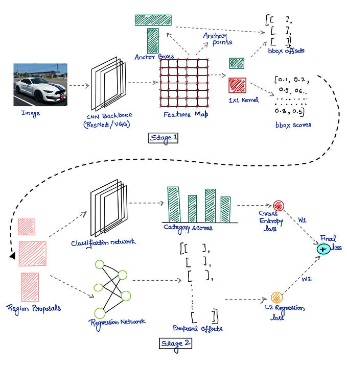
2. Region Proposal Network (RPN)
2. 지역 제안 네트워크(RPN)

In Faster R-CNN, both classification and bounding box regression happen twice — once in the Region Proposal Network (RPN) and again in the Faster RCNN after ROI pooling
Faster R-CNN에서는 분류 및 경계 상자 회귀가 두 번 발생합니다 . 한 번은 RPN(Region Proposal Network) 에서 발생하고 두 번은 ROI 풀링 후 Faster RCNN 에서 발생합니다.

Faster R-CNN introduced a Region Proposal Network (RPN), which completely changed how region proposals were generated in object detection. Before RPN, Fast R-CNN used Selective Search, which was slow and static (i.e., it didn’t improve over time). RPN learns to propose better regions dynamically, making the whole process faster and more accurate.
Faster R-CNN은 Region Proposal Network(RPN)를 도입했는데, 이는 객체 감지에서 영역 제안이 생성되는 방식을 완전히 바꾸었습니다. RPN 이전에 Fast R-CNN은 Selective Search를 사용했는데, 이는 느리고 정적 이었습니다(즉, 시간이 지나도 개선되지 않았습니다). RPN은 더 나은 영역을 동적으로 제안하는 방법을 학습하여 전체 프로세스를 더 빠르고 정확하게 만듭니다.

RPN replaces Selective Search with a trainable deep-learning-based approach, making region proposals part of the same neural network pipeline
RPN은 선택적 검색을 훈련 가능한 딥러닝 기반 접근 방식으로 대체하여 지역 제안을 동일한 신경망 파이프라인의 일부로 만듭니다.

RPN scans the feature maps using a small sliding window and predicts whether an object is present at each location. It does this using anchor boxes.
RPN은 작은 슬라이딩 윈도우를 사용하여 피처 맵을 스캔 하고 각 위치에 객체가 있는지 예측합니다. 앵커 박스를 사용하여 이를 수행합니다.

• What are anchor boxes?  앵커 박스란 무엇인가요?
• These are predefined bounding boxes of different sizes and aspect ratios.
  이는 다양한 크기와 종횡비를 갖는 미리 정의된 경계 상자 입니다.
• Each location on the feature map has multiple anchor boxes (e.g., 9 anchors per location).
  피처 맵의 각 위치에는 여러 개의 앵커 상자가 있습니다(예: 위치당 앵커 9개 ).
• The model predicts which anchor boxes contain objects and how to refine them.
  이 모델은 어떤 앵커 상자 에 객체가 포함되어 있는지 예측하고 이를 어떻게 세분화할지를 예측합니다.

Example:  예:
Imagine we have an image of a car. The RPN places anchor boxes of different shapes and sizes all over the feature map. Some boxes may be over the car, some may not. The network learns to pick the best boxes and refine their coordinates.
자동차 이미지가 있다고 가정해 보겠습니다. RPN은 피처 맵 전체에 다양한 모양과 크기 의 앵커 상자를 배치합니다. 일부 상자는 자동차 위에 있고, 일부는 그렇지 않을 수 있습니다. 네트워크는 최상의 상자를 선택 하고 좌표를 정제하는 법 을 배웁니다 .

Training of RPN  RPN의 훈련

To train the RPN, we need a loss function that tells the network:
RPN을 훈련하려면 네트워크에 다음 내용을 알려주는 손실 함수가 필요합니다.

• Which anchor boxes are good (foreground) and which are bad (background)?
  어떤 앵커 상자가 좋고(전경) 어떤 앵커 상자가 나쁩니까(배경)?
• How to adjust the anchor boxes to fit objects better?
  객체에 더 잘 맞도록 앵커 상자를 조정하는 방법은 무엇인가요?

The RPN has two outputs per anchor box:
RPN에는 앵커 박스당 2개의 출력이 있습니다.

1. Classification Output (Object vs. Background)
   분류 출력 (객체 대 배경)

• It classifies whether the anchor contains an object or not.
  앵커에 객체가 포함되어 있는지 여부를 분류합니다.

2. Bounding Box Regression Output (Refining the Box)
2. 바운딩 박스 회귀 출력 (박스 정제)

• It predicts small adjustments (x, y, width, height) to make the anchor box fit the object better.
  앵커 박스가 개체에 더 잘 맞도록 작은 조정(x, y, 너비, 높이)을 예측합니다.

The RPN Loss Function has two parts:
RPN 손실 함수는 두 부분으로 구성됩니다.

1. Classification Loss (Binary Cross-Entropy Loss)
   분류 손실(바이너리 크로스 엔트로피 손실)

• It tells the network how well it distinguishes objects from the background.
  이는 네트워크가 객체와 배경을 얼마나 잘 구별하는지를 알려줍니다.
• If an anchor box has an IoU > 0.7 with a ground truth box → It’s a positive example
  앵커 박스에 실제값 박스와 함께 IoU > 0.7이 있는 경우 → 이는 긍정적인 예입니다.
• If an anchor box has an IoU < 0.3 → It’s a negative example (background)
  앵커박스에 IoU < 0.3이 있는 경우 → 부정적인 예(배경)입니다 .
• If it’s in between, we ignore it.
  그 중간에 있는 것은 무시합니다.

2. Regression Loss (Smooth L1 Loss)
2. 회귀 손실(Smooth L1 Loss)

• It helps the network refine the anchor box coordinates to match objects better.
  네트워크가 앵커 박스 좌표를 정제하여 객체를 더 잘 일치시키는 데 도움이 됩니다.

3. ROI Pooling (Region of Interest Pooling)
3. ROI 풀링(ROI Pooling) (관심 영역 풀링)

• Purpose: Converts region proposals into fixed-size feature maps for classification and bounding box regression.
  목적 : 분류 및 경계 상자 회귀를 위해 영역 제안을 고정 크기의 특징 맵으로 변환합니다.
• Input:
  입력 :
• Feature Maps from CNN.
  CNN의 피처 맵 .
• Region Proposals from RPN.
  RPN의 지역 제안 .
• Output: Fixed-size feature maps (e.g., 7x7), regardless of the proposal’s original size.
  출력 : 제안의 원래 크기에 관계없이 고정 크기의 기능 맵(예: 7x7)입니다.

Example  예
A bounding box around a cat’s head might have different dimensions than a box around the full cat, but ROI Pooling converts them into the same fixed size for the next stage.
고양이 머리 주위의 경계 상자는 고양이 몸 전체를 둘러싼 상자와 크기가 다를 수 있지만, ROI 풀링은 이를 다음 단계에서 동일한 고정 크기 로 변환합니다.

4. Final Classifier & Bounding Box Regressor
4. 최종 분류기 및 경계 상자 회귀기

• Purpose:
  목적 :
• Classifier: Determines what object is inside each bounding box.
  분류기 : 각 경계 상자 내부에 어떤 개체가 있는지 판별합니다.
• Bounding Box Regressor: Refines the box’s position for better accuracy.
  경계 상자 회귀기 : 정확도를 높이기 위해 상자의 위치를 ​​조정합니다.
• Input: Fixed-size feature maps from ROI Pooling.
  입력 : ROI 풀링의 고정 크기 피처 맵.
• Output:
  출력 :
• Class Label (e.g., “Cat”)
  클래스 레이블(예: "고양이")
• Refined Bounding Box Coordinates
  정제된 바운딩 박스 좌표

Example  예

• The model might classify a region as a “Cat” with 92% confidence.
  이 모델은 92%의 신뢰도로 지역을 "고양이" 로 분류할 수 있습니다.
• The bounding box regressor fine-tunes the box so it tightly fits around the cat.
  경계 상자 회귀자는 상자가 고양이 주위에 꼭 맞도록 미세 조정합니다.

How are anchor boxes generated on the feature maps in the RPN?
RPN의 피처 맵에서 앵커 상자는 어떻게 생성됩니까?

1. Sliding Window Over Feature Map
1. 피처 맵 위의 슬라이딩 윈도우

• Faster R-CNN does NOT generate boxes randomly.
  Faster R-CNN은 무작위로 상자를 생성하지 않습니다 .
• It places anchor boxes at each location in the feature map (not the original image).
  피처 맵의 각 위치에 앵커 상자를 배치합니다 (원본 이미지가 아님).
• A location refers to the center of a cell in the feature map.
  위치는 피처 맵에서 셀의 중심 을 나타냅니다.
• If the feature map is 50×50, there are 50×50 = 2500 locations where anchor boxes can be placed.
  피처 맵이 50×50 이면 앵커 상자를 배치할 수 있는 위치는 50×50 = 2500개 입니다.
• At each of these 2500 locations, multiple anchor boxes (with different sizes and aspect ratios) are placed.
  이 2500개의 각 위치 에는 여러 개의 앵커 상자(크기와 종횡비가 다름)가 배치됩니다.
• Each feature map has its own set of anchor boxes.
  각 피처 맵에는 고유한 앵커 상자 세트가 있습니다.
  The anchor boxes are scaled based on the feature map size.
  앵커 상자의 크기는 피처 맵 크기에 따라 조정됩니다 .
  Using multiple feature maps helps in detecting objects at different scales
  여러 개의 기능 맵을 사용하면 다양한 크기의 객체를 감지하는 데 도움이 됩니다.
• This is done using a sliding window mechanism that moves across the feature map.
  이 작업은 피처 맵을 따라 움직이는 슬라이딩 윈도우 메커니즘을 사용하여 수행됩니다.

Analogy:  유추:
Imagine you have a grid over the image and at each grid point, you place several rectangular boxes of different sizes and shapes.
이미지 위에 격자를 놓고, 각 격자점에 크기와 모양이 다른 직사각형 상자를 여러 개 배치한다고 상상해보세요.

2. Multiple Anchor Boxes Per Location
2. 위치당 여러 앵커 박스

• Each location in the feature map gets multiple anchor boxes of different sizes and aspect ratios.
  피처 맵의 각 위치에는 크기와 종횡비가 다른 여러 앵커 상자가 있습니다.
• This helps detect objects of different scales and shapes.
  이는 다양한 크기와 모양의 물체를 감지하는 데 도움이 됩니다.

What do these boxes vary in?
이 상자들은 어떤 점에서 다릅니까?
1. Scale (Size): Small, Medium, Large objects
1. 규모(크기): 작은, 중간, 큰 물체
2. Aspect Ratio: Square, Tall, Wide objects
2. 종횡비: 정사각형, 키가 큰 개체, 넓은 개체

Example: Suppose we use 3 different scales and 3 different aspect ratios at each location.
예: 각 위치에서 3개의 서로 다른 크기 와 3개의 서로 다른 종횡비를 사용한다고 가정해 보겠습니다.

• Scale: Small (32×32), Medium (64×64), Large (128×128)
  크기: 소형(32×32), 중형(64×64), 대형(128×128)
• Aspect Ratios: 1:1 (square), 1:2 (tall), 2:1 (wide)
  종횡비: 1:1(정사각형), 1:2(높이), 2:1(너비)
• Total Anchors Per Location: 3 scales × 3 ratios = 9 anchor boxes per location
  위치당 총 앵커: 3개 스케일 × 3개 비율 = 위치당 9개 앵커 상자

Real-World Example:  실제 세계의 예:
Think of different-sized picture frames placed all over a wall to make sure they fit different-sized photos. Some are square, some are wide, and some are tall.
다양한 크기의 사진 프레임을 벽 전체에 배치하여 다양한 크기의 사진에 맞는지 확인하세요. 일부는 정사각형이고, 일부는 넓고, 일부는 키가 큽니다.

3. Why Are These Anchor Boxes Placed on a Feature Map and Not the Original Image?
3. 이러한 앵커 상자가 원본 이미지가 아닌 피처 맵에 배치되는 이유는 무엇입니까?

• Directly working on an image would require generating millions of boxes.
  이미지 작업을 직접 하려면 수백만 개의 상자를 생성해야 합니다.
• Instead, Faster R-CNN first applies a CNN (like ResNet or VGG) to extract a feature map, which is much smaller than the original image.
  대신, Faster R-CNN은 먼저 CNN(ResNet이나 VGG와 같은)을 적용하여 원본 이미지보다 훨씬 작은 피쳐 맵을 추출합니다.
• The anchor boxes are then placed on this smaller feature map to save computation time.
  그런 다음 계산 시간을 절약하기 위해 앵커 상자가 이 작은 피처 맵 에 배치됩니다.

Example:  예:

• Suppose the original image is 800×800 pixels.
  원본 이미지가 800×800픽셀 이라고 가정합니다.
• After passing through a CNN, the feature map is reduced to 50×50 pixels.
  CNN을 거친 후, 피처 맵은 50×50픽셀 로 줄어듭니다.
• If we place 9 anchor boxes per location, we get 50×50×9 = 22,500 anchor boxes instead of millions if done directly on the image.
  위치당 앵커 박스를 9개 배치하면 이미지에 직접 배치할 경우 수백만 개가 아닌 50×50×9 = 22,500개의 앵커 박스를 얻게 됩니다.

Analogy:  유추:
Instead of searching for small objects pixel-by-pixel (slow), we search at a coarser level (faster) and refine later.
작은 객체를 픽셀 단위 로 검색하는 것(느림) 대신, 더 거친 수준 (빠름)으로 검색한 다음 나중에 세부적으로 처리합니다.

Why is faster RCNN faster? It is using sliding window to generate anchor boxes and it has to train 2 classification network and bbox regression (one in RPN and other after ROI pooling); so it should be slow, but then why is it faster than RCNN and fast RCNN?
Faster RCNN이 왜 더 빠른가요? 슬라이딩 윈도우를 사용하여 앵커 박스를 생성하고 2개의 분류 네트워크와 bbox 회귀(하나는 RPN에서, 다른 하나는 ROI 풀링 후)를 훈련해야 하므로 느릴 수밖에 없지만, 왜 RCNN과 fast RCNN보다 빠른가요?

You’re absolutely right! At first glance, Faster R-CNN should be slow because:
당신 말이 전적으로 맞아요! 언뜻 보기에 Faster R-CNN은 다음과 같은 이유로 느릴 겁니다.

1. Sliding Window for Anchors: It generates thousands of anchor boxes per image.
   앵커용 슬라이딩 윈도우: 이미지당 수천 개의 앵커 상자를 생성합니다.
2. Two-Step Processing: First in the RPN, then again in the Fast R-CNN head (classification & bbox regression).
   2단계 처리: 먼저 RPN에서, 그다음 다시 Fast R-CNN 헤드에서 처리(분류 및 Bbox 회귀).

Yet, it is called “Faster R-CNN” because of these key optimizations:
그러나 이러한 핵심 최적화 때문에 " Faster R-CNN"이라고 불립니다.

1. Sharing CNN Features for RPN & Detection
1. RPN 및 감지를 위한 CNN 기능 공유

Instead of processing the image separately for RPN and classification, Faster R-CNN shares the same CNN feature maps between both stages.
RPN과 분류를 위해 이미지를 별도로 처리하는 대신, Faster R-CNN은 두 단계 간에 동일한 CNN 기능 맵을 공유합니다 .

What this means:  이는 무엇을 의미합니까?

• The backbone CNN (like ResNet, VGG) extracts features just once from the image.
  백본 CNN(ResNet, VGG와 유사)은 이미지에서 특징을 한 번만 추출합니다 .
• The same feature maps are used for both RPN (to generate proposals) and Fast R-CNN (to classify and refine proposals).
  동일한 특징 맵이 RPN(제안 생성용) 과 Fast R-CNN(제안 분류 및 개선용)에 모두 사용됩니다.
• This eliminates redundant computation, making the process much faster.
  이를 통해 중복된 계산이 제거되어 프로세스가 훨씬 더 빨라집니다.

Impact:  영향:
Reduces computation time significantly.
계산 시간이 크게 단축됩니다.
Makes Faster R-CNN much faster than RCNN & Fast R-CNN.
Faster R-CNN을 RCNN 및 Fast R-CNN보다 훨씬 빠르게 만듭니다.

2. Why is RPN Faster than Selective Search?
2. RPN이 선택적 검색보다 빠른 이유는 무엇입니까?

Problem with Selective Search (Fast R-CNN)
선택적 검색(Fast R-CNN)의 문제

In Fast R-CNN, region proposals were generated using Selective Search, which is a slow and handcrafted algorithm.
Fast R-CNN에서는 선택적 검색(Selective Search)을 사용하여 영역 제안을 생성했는데, 이는 느리고 수작업으로 만들어진 알고리즘 입니다.
It looks at color, texture, and other image properties to group similar regions — this is computationally expensive and not trainable.
유사한 영역을 그룹화하기 위해 색상, 질감 및 기타 이미지 속성을 살펴봅니다. 이는 컴퓨팅 측면에서 비용이 많이 들고 학습이 불가능합니다 .

Solution in Faster R-CNN: Trainable RPN
Faster R-CNN의 솔루션: 훈련 가능한 RPN

Faster R-CNN replaces Selective Search with a small neural network called the Region Proposal Network (RPN).
Faster R-CNN은 선택적 검색을 RPN(Region Proposal Network) 이라는 작은 신경망으로 대체합니다 .

RPN is a lightweight CNN that slides over feature maps and predicts where objects might be.
RPN은 피쳐 맵을 따라 움직이며 객체가 어디에 있을 수 있는지 예측하는 가벼운 CNN입니다.

Since it runs inside the neural network itself, it learns to improve proposal quality over time instead of using fixed rules like Selective Search.
신경망 자체 내부에서 실행되므로 선택적 검색과 같은 고정된 규칙을 사용하는 대신 시간이 지남에 따라 제안 품질을 개선하는 방법을 학습합니다 .

Example:  예:

• Imagine you’re looking for cars in a parking lot.
  주차장에서 차를 찾고 있다고 상상해 보세요.
• Selective Search checks every single patch of the image manually and does this iteratively — this takes a lot of time.
  선택적 검색은 이미지의 모든 패치를 수동으로 반복적으로 확인하므로 시간이 많이 걸립니다.
• RPN quickly scans the whole scene at once and picks out likely locations, making it much faster.
  RPN은 전체 장면을 한 번에 빠르게 스캔 하고 가능성 있는 위치를 골라내므로 작업이 훨씬 더 빨라집니다.

3: Why Doesn’t Sliding Window Make RPN Slow?
3: 슬라이딩 윈도우가 RPN을 느리게 만들지 않는 이유는 무엇인가?

Problem with Traditional Sliding Window
기존 슬라이딩 윈도우의 문제점

The old way of detecting objects was to slide a small window across the entire image at multiple scales.
이전에 객체를 감지하는 방법은 여러 크기에 맞춰 전체 이미지에 작은 창을 밀어 넣는 것이었습니다.
This meant checking millions of possible locations, making it very slow.
이는 수백만 개의 가능한 위치를 확인해야 한다는 의미로, 매우 느렸습니다 .

Solution in Faster R-CNN: Anchor Boxes
Faster R-CNN의 솔루션: 앵커 박스

Instead of checking every possible region from scratch, RPN uses predefined anchor boxes at different sizes and aspect ratios.
RPN은 모든 가능한 영역을 처음부터 검사하는 대신, 다양한 크기와 종횡비의 미리 정의된 앵커 상자를 사용합니다.
These anchor boxes are placed at fixed positions on the feature map, and RPN only needs to adjust them to fit actual objects.
이러한 앵커 상자는 피처 맵의 고정된 위치에 배치되고 , RPN은 실제 객체에 맞게 앵커 상자를 조정하기만 하면 됩니다 .

Example:  예:

• Imagine you are a tailor making custom suits.
  당신이 맞춤형 양복을 만드는 재단사 라고 상상해보세요.
• Instead of measuring every person from scratch, you start with pre-made standard sizes (S, M, L, XL) and then make small adjustments.
  모든 사람을 처음부터 측정하는 대신, 미리 만들어진 표준 사이즈(S, M, L, XL)를 기준으로 시작하여 작은 조정을 합니다.
• Anchor boxes work the same way — they provide a starting point for object locations, so the model doesn’t need to check everything from scratch.
  앵커 상자도 같은 방식으로 작동합니다. 즉, 객체 위치에 대한 시작점을 제공하므로 모델이 모든 것을 처음부터 확인할 필요가 없습니다 .

Result:  결과:

• This dramatically reduces the number of regions the model needs to process.
  이를 통해 모델이 처리해야 하는 지역의 수가 극적으로 줄어듭니다 .
• Instead of millions of possibilities, it only fine-tunes a few thousand anchor boxes — making it much faster than sliding window approaches.
  수백만 가지의 가능성 대신, 몇 천 개의 앵커 박스만 미세 조정하므로 슬라이딩 윈도우 방식보다 훨씬 빠릅니다 .