Avoiding Overfitting and Colinearity with Regularization

Fighting 2 very important problems in quant finance

2 of the most common problems we face when building trading models are overfitting and colinearity. Regularization is a technique that we can use to combat both of those problems.

More broadly, regularization is a process that converts the answer of a problem to a simpler one.
This can be done in multiple different ways. Some explicit regularization techniques are penalties and constraints. Implicit regularization techniques are early stopping, robust loss functions, discarding outliers etc.

Bias-variance tradeoff tells us that as we increase regularization to learn broader patterns in our data our variance decreases but therefore our bias (inaccuracy) increases.

https://en.wikipedia.org/wiki/Bias%E2%80%93variance_tradeoff

---

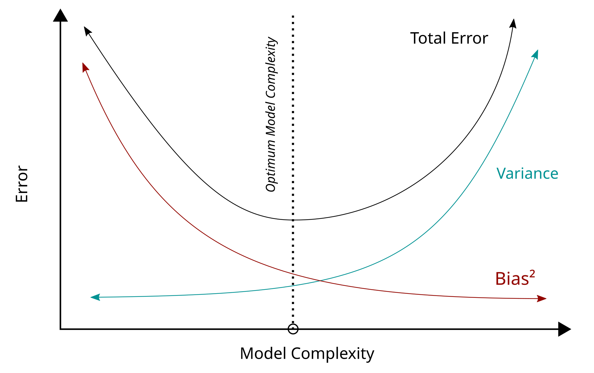
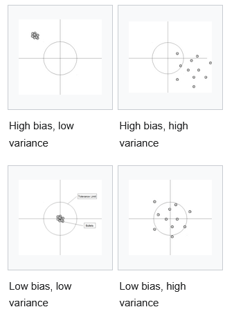
Table of Content

1. Norm Penalization and Constraints

2. Lasso, Ridge and Elastic Net Regression

3. Polynomial Regression

4. Model Selection

5. Robust Covariance Matrix

6. Final Remarks

---

Norm Penalization and Constraints

First let’s understand the definition of a norm:

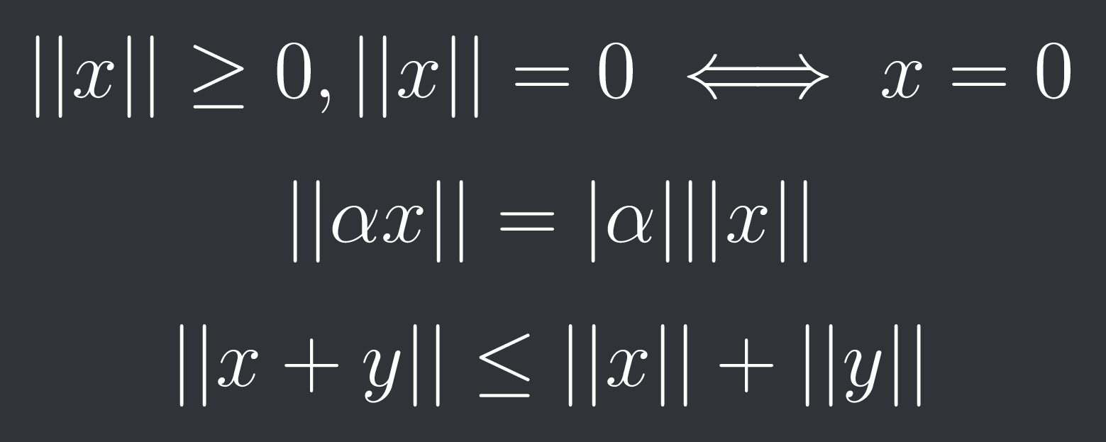
Given a vector space V (usually just the set of real numbers) over the real or complex numbers. A function || * || : V → R is called a norm, if for all x,y in V and alpha in R (or C) we have:

1. Positive definiteness

2. Absolute homogeneity

3. Triangle inequality

Norms have the nice property that they are convex which means we can use them in convex optimization problems.

A broader group of functions are quasi-norms for which we have a weaker form of the triangle inequality:

Quasi-norms are not necessarily convex so we don’t use them in optimization problems as often.

By far the 2 most popular norms in regularization are the L1- and L2-norm.
They are defined as follows:

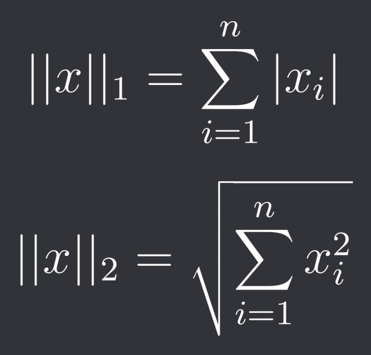
So the L1-norm is the sum of the absolute values of the components and the L2-norm is the sum of the squares of the components.

Another norm that is often used is the L-infinity norm defined as:

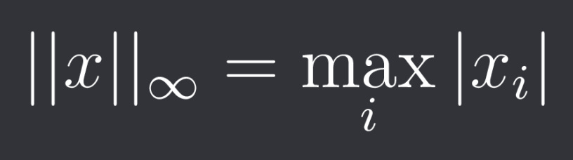
They are part of broader group of (discrete) Lp norms:

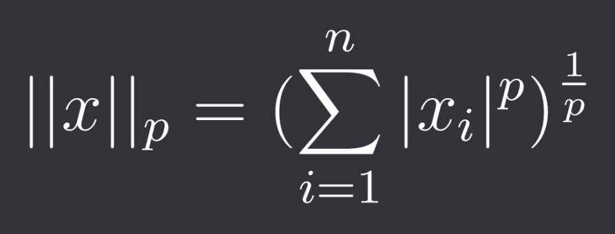
Where p >= 1.

The L-infinity norm is actually the limit of those norms against infinity.

For 0 < p < 1 we obtain quasi-norms. One example is the L-2/3 quasi-norm.

Let’s plot ||x||_p <= 1 (the unit ball) for different values of p for x 2-dimensional:

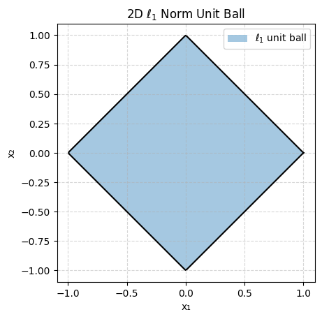
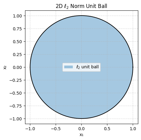
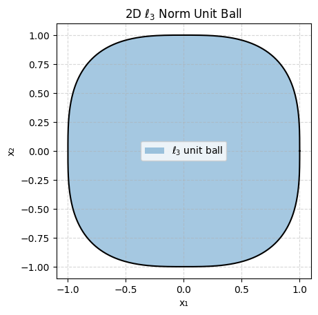
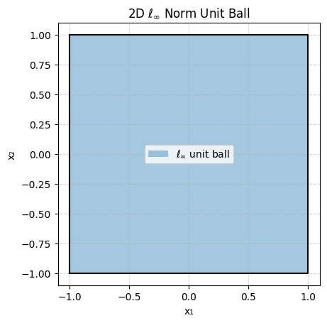
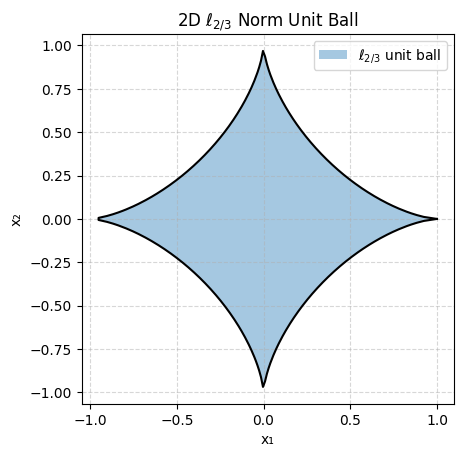
As you can see some are very pointy and some are smooth which will be important depending on what goal we are trying to achieve.

Let’s say you are constructing a trading portfolio with an asset universe of 100 assets.
Now you don’t want your portfolio to actually contain 100 different assets so you have the constraint #Assets <= 10. Unfortunately this is not a convex constraint so you wouldn’t be able to solve it as easily anymore.

This is where “pointy” norms like L1 come in. While not guaranteed the optimal points are often at the edge points and with L1 this coincides with variables being exactly 0. And because L1 is convex we can use the convex approximated ||x||_1 <= 10.

If we instead use something like the L2-norm in the constraint then we usually don’t get exact 0s but very small weights. This is often more useful when building forecasting models for example where we don’t want to completely get rid of predictors.

Another way we can use norms is as a penalization in the objective function.
So instead of minimizing the variance of a portfolio you could minimize variance - lambda * ||weights||_1 for example where lambda controls how much regularization you want.

Such constraints and penalizations are commonly used in portfolio optimization where we want sparse portfolios, maximum leverage etc.

---

Lasso, Ridge and Elastic Net Regression

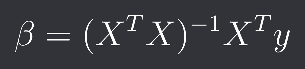
In standard multiple linear regression you solve the optimization problem:

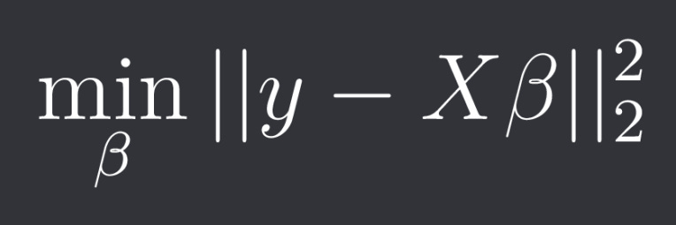
Where y is your target vector with n samples, X is your feature matrix with n samples and p features and beta are your p coefficients. The closed-form solution is:

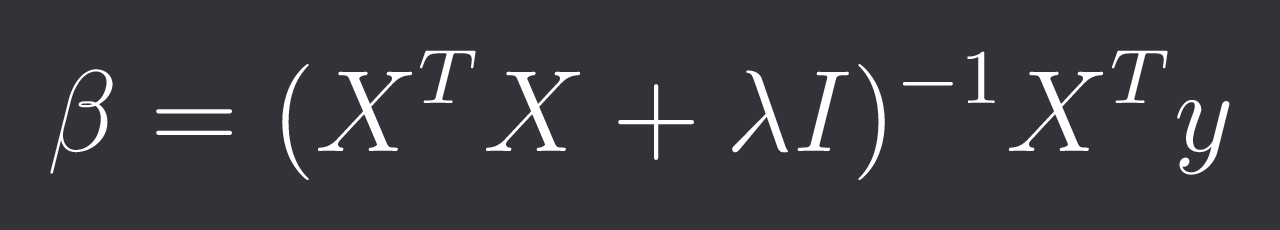
With ridge regression we penalize the square of the L2-norm like described in the previous chapter:

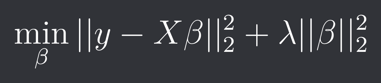
This actually has a closed-form solution:

In lasso regression we penalize the L1-norm:

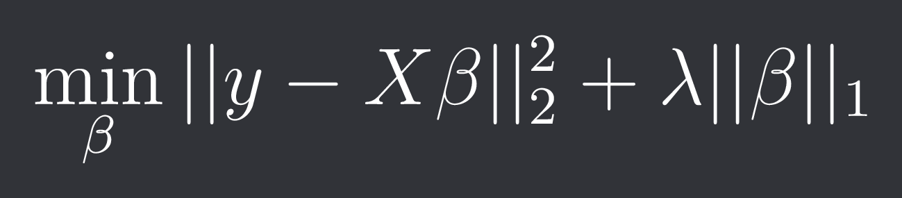
The L1-norm is non-differentiable at 0 so we can’t give a closed-form solution so usually subgradient methods and coordinate descent are used to find a beta.

This gives those 2 regularizations the name ridge regularization and lasso regularization.

Lastly we have Elastic Net regression which simply combines the 2 penalizations:

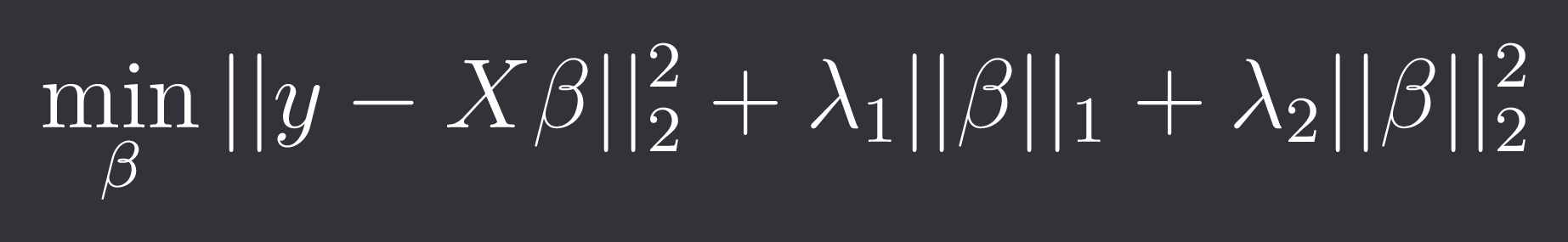
Because of the non-differentiability of the L1-norm there is also no closed-form solution.

Those 3 regression techniques are able to fight colinearity. How so?
Imagine you have variable 1. You now introduce another variable 2 which is highly correlated to 1. It probably won’t improve the fit all that much but because we now have a new parameter the norm of all our parameters is gonna increase.
Because we are penalizing the norm it’s likely that ignoring the second parameter or choosing a small value will result in lower accuracy but we’ve gotten (mostly) rid of a colinear parameter.

Lasso, Ridge and Elastic Net are really big and important topic in quant finance and deserve their own article so I will not go into them much further in this article (since this article is about general uses of regularization anyway).

---

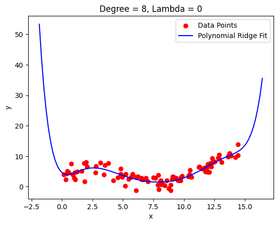
Polynomial Regression

Given a bunch of data points we can fit a polynomial through them that minimizes the sum of squared errors.

Now the problem is:

• Low degree polynomials often underfit

• High degree polynomials shoot off and wildy oscillate between points

The solution is to use high degree polynomials with regularized coefficients.

Our optimization problem is thus of the form:

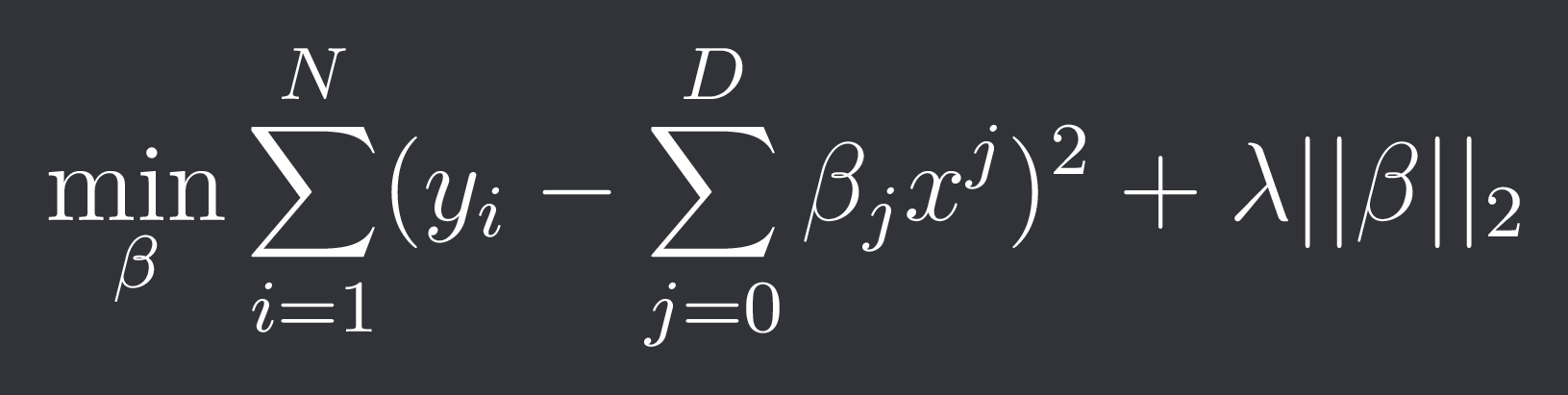
where D is the degree of the polynomial.
Note: The constants coefficient beta_0 is often ignored in the regularization.
We could of course have chosen any other norm other than the L2-norm again but the L2-norm gives us a nice closed-form solution (see ridge regression).

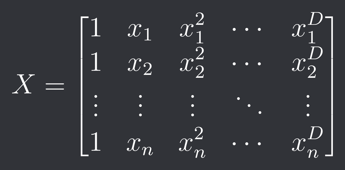
The feature matrix X in polynomial regression is a special case and is called the vandermonde matrix:

Here is the python code to compute polynomial regression with regularization:

def polynomial_regression_regularized(x, y, degree, alpha):
    X = np.vander(x, degree+1, increasing=True)

    I = np.eye(X.shape[1])
    I[0, 0] = 0 # Don't regularize intercept

    beta = np.linalg.inv(X.T @ X + alpha * I) @ X.T @ y

    return beta

Let’s look at an example:

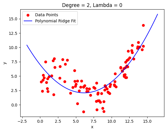
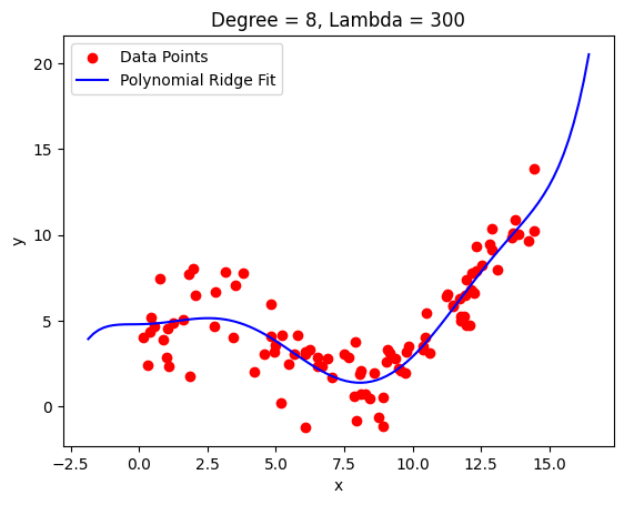
We still get a fairly good fit with the same order polynomial but have a much smoother curve now that doesn’t shoot off right away.

This is particularly useful if you don’t have very sudden changes in the shape of your data. You can see how the fit around 2.5 got worse because it got smoothed out there.

---

Model Selection

Let’s say you have a bunch of models that you’ve already fit and you want to decide which is the best one.

Simply picking the best fitting one is not the best idea as you will likely just overfit. You want some performance measure that takes into account the complexity of the model.

So far we’ve done that by penalizing the norm of the model coefficients but there are other techniques as well like AIC and BIC that penalize the total number of parameters you have.

We can do this even though the number of parameters is not convex since we’ve fit the different models without any regularization and *then* take into account model complexity when deciding which one to use.

If you wanna learn more about model selection I recommend reading my article on it:

---

Robust Covariance Matrix

Estimating a covariance matrix is not such an easy task. Sure we can just compute the sample covariance matrix but especially if we have a lot of assets and not a lot of samples it’s gonna be super fragile (high variance).

We can “shrink” the sample covariance matrix S towards some target matrix T (for example the identity or the diagonal of S) using a parameter lambda in [0, 1]:

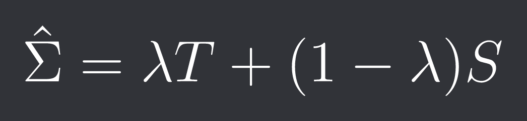
The larger we choose lambda the more stable our covariance matrix will become but the more biased it will be.

There are 2 popular methods for choosing an optimal lambda:

Oracle Approximating Shrinkage (OAS):

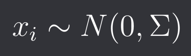
We assume that our observations x_i (returns at time i) are drawn from a multivariate normal distribution:

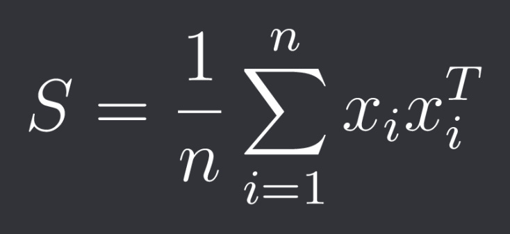
The sample covariance matrix S is therefore:

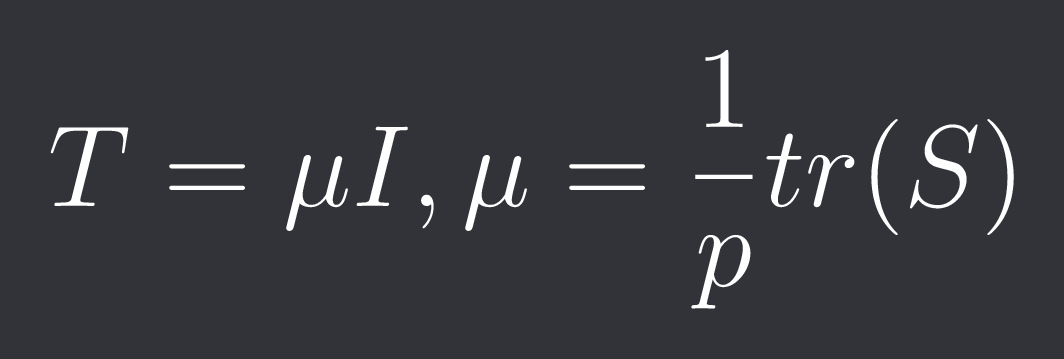
The target matrix T is the identity matrix scaled by the average sample variance:

Our optimal lambda solves the following minimization problem:

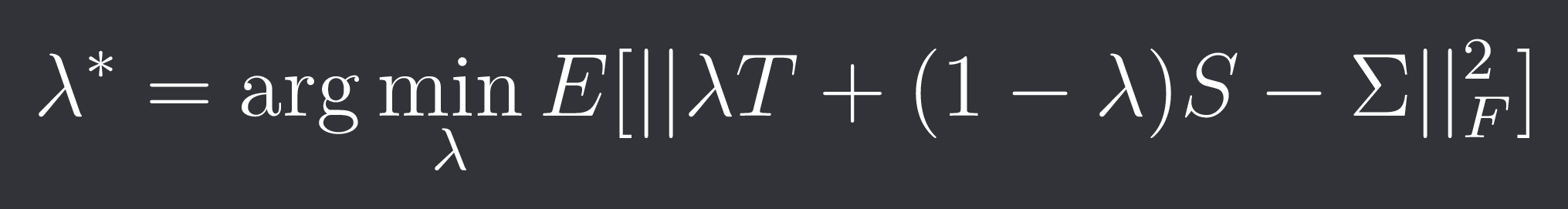
Here ||*||_F is the so called Frobenius-norm which is a matrix norm.

Note: We can induce a matrix norm from a vector norm in the following way:

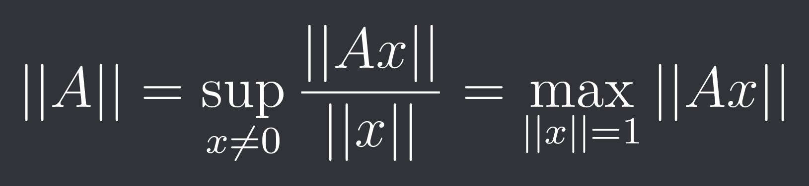
The Frobenius-norm is a matrix norm that is not induced by a vector norm.
It's defined as:

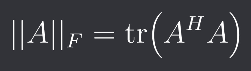
Where H is the conjugate transpose which is simply the regular transpose T if A is real.

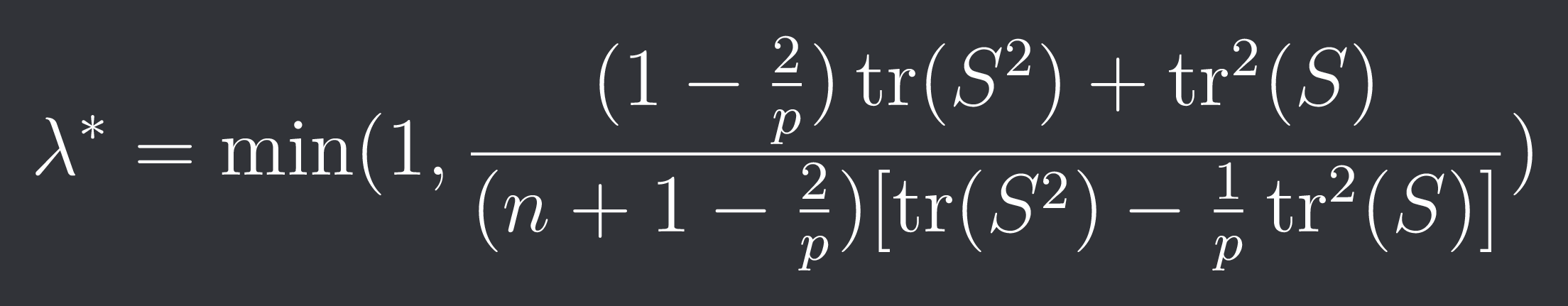
Under the gaussian assumption the optimal lambda is:

Ledoit-Wolf Shrinkage:

We no longer assume normality. Therefore our sample covariance is:

The target matrix T is the same as in OAS. The optimization is also the same.

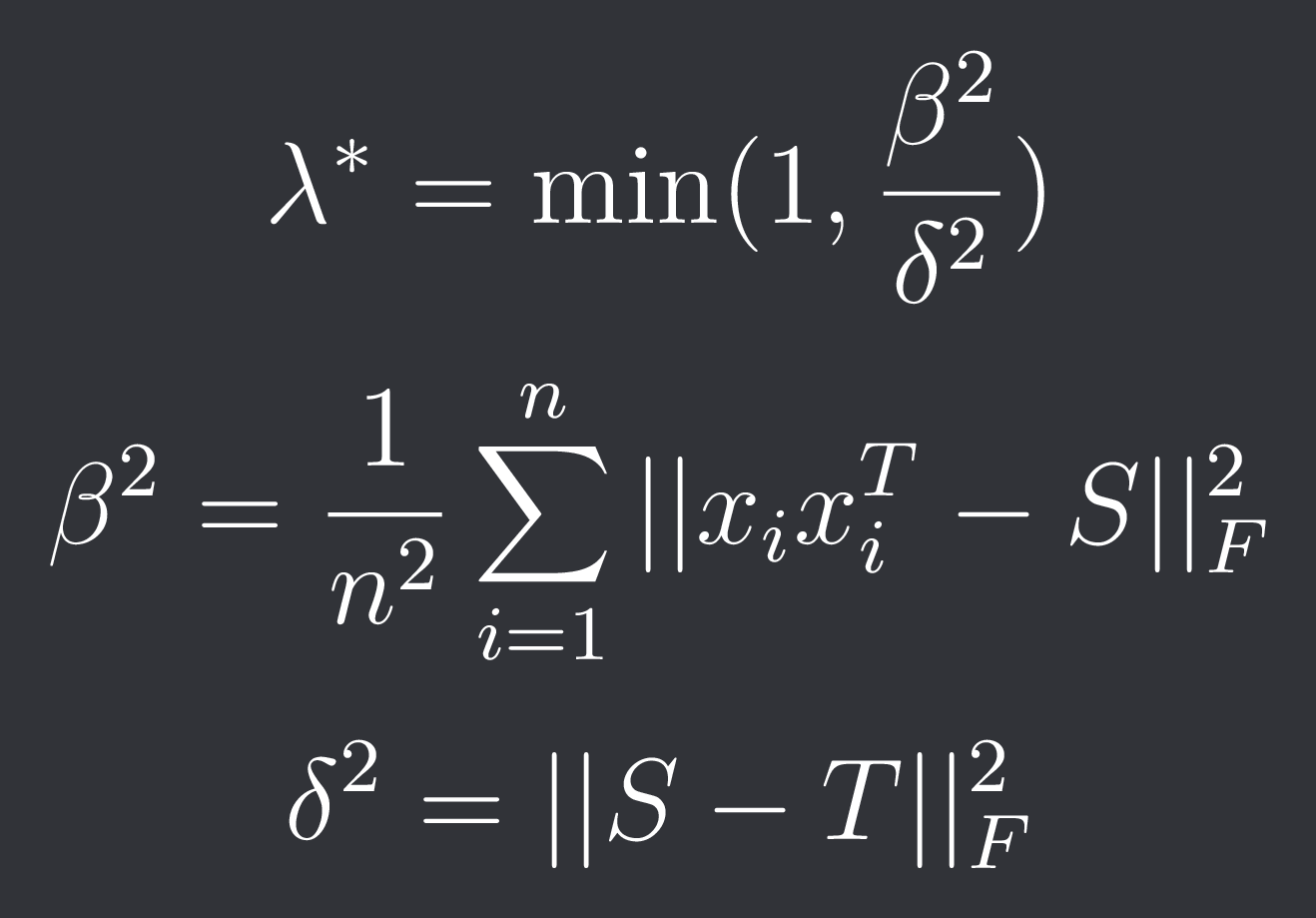
The optimal lambda is then given by:

---

Final Remarks

There are many many more applications of regularization. You could penalize the number of leaves in a decision tree or you could deactivate certain nodes when training a neural network etc.

This article should have given you a good overview and a good intuitive idea by looking at a few specific examples of what regularization is about.

Discord: https://discord.gg/X7TsxKNbXg