90. Python
概率论和统计学基础#
90. Fundamentals of Probability Theory and Statistics in Python
90.1. 介绍# 90.1. Introduction
概率论是一种用于表示不确定性声明的数学框架。很多机器学习算法的设计都会依赖于对数据的概率假设。同样,我们还可以使用概率和统计的相关知识,从理论上分析我们提出的
AI 系统的行为。
本实验主要是对机器学习中常用的概率论和统计学习方法进行讲述。
Probability theory is a mathematical framework used to represent statements of uncertainty. The design of many machine learning algorithms relies on probabilistic assumptions about the data. Similarly, we can use knowledge of probability and statistics to theoretically analyze the behavior of the AI systems we propose. This experiment mainly discusses the commonly used probability theory and statistical learning methods in machine learning.
90.2. 知识点# 90.2. Knowledge Point #
概率公式 Probability formula
随机变量 Random variable
概率分布 Probability distribution
数学期望 Mathematical expectation
方差、标准差和协方差 Variance, Standard Deviation, and Covariance
假设检验 Hypothesis testing
概率论是一种用于表示不确定性声明的数学框架。很多机器学习算法的设计都会依赖于对数据的概率假设。同样我们还可以使用概率和统计的相关知识,从理论上分析我们提出的
AI
系统的行为。接下来,让我们介绍一下概率论中最为重要的几个概率公式。
Probability theory is a mathematical framework used to represent statements of uncertainty. The design of many machine learning algorithms relies on probabilistic assumptions about the data. Similarly, we can use related knowledge of probability and statistics to theoretically analyze the behavior of our proposed AI systems. Next, let's introduce some of the most important probability formulas in probability theory.
90.3. 条件概率# 90.3. Conditional Probability
条件概率即在某个条件之下的概率。如当事件
Conditional probability is the probability under a certain condition. For example, when event
条件概率
The formula for calculating the conditional probability
举个例子,一个盒子里混有 100
只新旧乒乓球,且这些乒乓球中有红色和黄色两种。分类如下:
For example, a box contains 100 mixed new and old ping pong balls, and these ping pong balls come in two colors: red and yellow. The classification is as follows:
黄色 |
白色 |
|
|---|---|---|
新 |
40 |
30 |
旧 |
20 |
10 |
如果我从盒子中取出了一个球,已知该球为
黄色,那么请问该球为新球的概率是多少呢?
If I took a ball out of the box, and it is known that the ball is yellow, then what is the probability that the ball is new?
我们可以从上表看出,这个黄色球为新球的概率为
We can see from the above table that the probability of this yellow ball being a new ball is
当然,我们也可以使用上面讲到的条件概率的方法: Of course, we can also use the conditional probability method mentioned above:
设事件 A ={从盒子中随机取一个球,该球为黄球},则根据上表可得
Let event A = {randomly drawing a ball from the box, the ball is yellow}, then according to the above table, we get
设事件 B
={从盒子中随机取一个球,该球是新球},则根据上表可知,取出的球为黄色新球的概率为:
Let event B = {a ball is randomly taken from the box, and the ball is a new ball}, then according to the above table, the probability that the taken ball is a new yellow ball is:
则取出一个球为黄色球,那么该球也为新球的概率如下:
If a ball is drawn and it is a yellow ball, then the probability that this ball is also a new ball is as follows:
请注意,这里的事件
Please note that the event
90.4. 全概率公式# 90.4. The Law of Total Probability
定义:设
Definition: Let
全概率公式可以通过下图进行解释: The total probability formula can be explained through the following diagram:
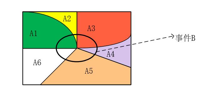
当我们直接求取
When it is very difficult to directly obtain
然后再根据条件概率公式,将上列式子转换一下: Then, according to the conditional probability formula, convert the above expression:
这就是全概率公式的来历。该公式的主要思想就是,在计算
This is the origin of the total probability formula. The main idea of this formula is that when it is difficult to calculate
举一个简单的例子,假设某车间使用甲、乙、丙、丁四台机床。各个机床的次品率分别为
5%,4%,3%,3.5%,且它们各自的产品占了总产量的
20%,35%,25%,20%。现在把它们混在一起,问随机取出一个产品为次品的概率。
Take a simple example, suppose a workshop uses four machines: A, B, C, and D. The defect rates of each machine are 5%, 4%, 3%, and 3.5% respectively, and their products account for 20%, 35%, 25%, and 20% of the total output. Now, if they are mixed together, what is the probability that a randomly selected product is defective?
思路:根据题目描述,我们可以知道: Idea: Based on the problem description, we can know:
-
某个产品来自于某个机床的概率
The probability that a certain product comes from a certain machine tool is -
次品率
Defective rate
而我们现在需要求的是
What we need to find now is
import numpy as np

# 将百分数转为小数
pa = np.array([20.0, 35, 25, 20])*0.01
pb_A = np.array([5.0, 4, 3, 3.5])*0.01
# 利用全概率公式计算次品率:先相乘再求和
pb = np.sum(np.multiply(pa, pb_A))

print("总次品率为:{}%".format(pb*100))
总次品率为:3.85%
90.5. 贝叶斯公式# Bayes' Theorem
定义:设
Definition: Let
上式即为贝叶斯公式的推导,其实无论是全概率公式的推导还是贝叶斯公式的推导,他们的核心都是使用条件概率公式。
The above formula is the derivation of Bayes' theorem. In fact, whether it is the derivation of the total probability formula or the derivation of Bayes' theorem, their core is the use of the conditional probability formula.
贝叶斯公式和全概率公式的不同:假设这里存在几种方式来达到一个相同的目标,每种方式达到目标的概率不同。全概率公式就是用于计算最终能够达到该目标的概率值(即不管使用哪种方式)。而贝叶斯公式计算的是,已知目标已经达成的条件下,使用每种方式的概率。
The difference between Bayes' theorem and the law of total probability: Suppose there are several ways to achieve the same goal, each with a different probability of success. The law of total probability is used to calculate the final probability of achieving the goal (regardless of which method is used). Bayes' theorem, on the other hand, calculates the probability of using each method given that the goal has already been achieved.
还是拿上面机床加工产品举例,设抽出产品为次品为事件 B,第
Let's still take the example of machining products with the above machine tool. Let event B be the extraction of a defective product, event
假设现在还是将所有的产品混在一起,然后从中抽出一个产品。发现这个产品是次品,问该产品来自各个机床的概率
Assuming that all the products are still mixed together, and then one product is drawn from them. It is found that this product is defective. What is the probability that this product came from each machine tool?
根据题目,我们需要求的就是
According to the question, what we need to find is
# 根据贝叶斯公式,计算来自每个机床的概率
# 这里的 pb 可以通过全概率公式进行计算
pA_b = (pa*pb_A) / pb

for i in range(4):
    print("该产品来自第 {} 个机床的概率:{}".format(i+1, pA_b[i]))
该产品来自第 1 个机床的概率:0.25974025974025977
该产品来自第 2 个机床的概率:0.3636363636363637
该产品来自第 3 个机床的概率:0.1948051948051948
该产品来自第 4 个机床的概率:0.18181818181818185
90.6. 概率分布# 90.6. Probability Distribution
90.7. 数据的类型# 90.7. Data Types
在编程中,我们常常需要一些随机值(比如在模拟抛硬币时)。我们将这些存储随机值的变量称之为随机变量。
In programming, we often need some random values (for example, when simulating a coin toss). We call these variables that store random values random variables.
随机变量根据产生的数值范围不同,可以分成两种类型:
Random variables can be divided into two types based on the range of values they produce:
-
离散型随机变量:如果随机变量
Discrete random variable: If the random variable -
连续型随机变量:如果随机变量
Continuous random variable: If all possible values of the random variable
无论是哪种随机变量,它的产生原理就是给它的范围中的每个可取值赋予一个概率,然后根据概率随机给变量赋值。
No matter what kind of random variable it is, its generation principle is to assign a probability to each possible value within its range, and then randomly assign a value to the variable based on the probability.
描述所有可取值的概率函数又可以根据变量类型不同分为:
The probability functions of all possible values can also be divided according to different variable types:
-
概率质量函数:描述离散变量的可取值的概率函数。 Probability mass function: a probability function that describes the possible values of a discrete variable.
概率密度函数:描述连续型变量的概率分布函数。 Probability density function: describes the probability distribution function of continuous variables.
概率分布是指随机变量的概率规律。简单的说,概率分布描述了随机变量的每个可取值,所对应的概率。在模拟数据时,我们根据概率的不同,对数据的取值也不同。接下来,让我们来详细介绍一下常见的离散型概率分布和连续型概率分布函数。
A probability distribution refers to the probability law of a random variable. Simply put, a probability distribution describes the probability corresponding to each possible value of a random variable. When simulating data, we assign different values to the data based on different probabilities. Next, let's take a detailed look at common discrete probability distributions and continuous probability distribution functions.
注意,对于初学者,我们不必背下每个函数的具体形式。我们更应该了解的是每种分布函数的特点和适用范围。
Note that for beginners, we don't need to memorize the specific form of each function. What we should understand more are the characteristics and applicable scope of each distribution function.
90.8. 离散型概率分布# 90.8. Discrete Probability Distribution #
在生活中,有许多事件的结果往往只有两个。例如:抛硬币的结果(正面朝上或者朝下)、检查产品的质量(合格或不合格)、购买彩票(中奖或不中奖),以上这些事件都可以叫做伯努利实验。
In life, there are many events that often have only two outcomes. For example: the result of flipping a coin (heads or tails), checking the quality of a product (pass or fail), buying a lottery ticket (win or lose). All of these events can be called Bernoulli trials.
伯努利试验其实就是单次随机试验,且结果只有 0 或 1
两种,由科学家伯努利提出。伯努利实验产生的数据分布就是两点分布。
A Bernoulli trial is essentially a single random experiment with only two possible outcomes, 0 or 1, proposed by the scientist Bernoulli. The data distribution generated by a Bernoulli experiment is a two-point distribution.
二点分布:也就是我们最常见的 0-1
分布。服从该分布的变量只有 0 和 1
两种取值。该分布的概率质量函数如下:
Two-point distribution: This is also the most common 0-1 distribution. Variables that follow this distribution have only two possible values, 0 and 1. The probability mass function of this distribution is as follows:
其中
The possible values of
我们可以通过每个
We can generate random numbers based on the probability corresponding to each
def Bernoulli(lambd_a):
    p = np.random.rand()
    # 表示返回 1 的概率 为 lambda
    if(p < lambd_a):
        return 1
    else:
        return 0
我们可以利用上面函数进行抛硬币的模拟,假设抛 5 次硬币:
We can use the above function to simulate coin tossing, assuming 5 coin tosses:
for i in range(5):
    print("第{}次实验结果:".format(i+1))
    result = Bernoulli(0.5)  # 每面的结果概率相同
    if(result == 1):
        print("正面")
    else:
        print("反面")
第1次实验结果:
正面
第2次实验结果:
反面
第3次实验结果:
正面
第4次实验结果:
反面
第5次实验结果:
反面
二项分布:进行
Binomial distribution: The probability distribution of the number of times the result is 1 after conducting
如果一个实验每次成功的概率为
If the probability of success for each experiment is
其中
Among them,
其实上面的这个函数就是二项分布的概率质量函数。表示在进行
In fact, the above function is the probability mass function of the binomial distribution. It represents the probability of having
注意,通过两点分布返回的是一次抛一个硬币的实验结果(0 或
1)。通过二项分布返回的是每次实验抛
Note that the result returned by the Bernoulli distribution is the outcome of a single coin toss (0 or 1). The result returned by the binomial distribution is the number of heads when
当
When
虽然上面的式子较为复杂,但是不需要手动编写。我们可以使用
numpy.random.RandomState.binomial(n,
                      p,
                      size=None)
随机初始化 x 的值。
Although the above formula is relatively complex, it does not need to be manually written. We can use numpy.random.RandomState.binomial(n,
p,
size=None)
to randomly initialize the value of x.
该函数就是利用上面式子所提供的概率值,来随机初始化
The function uses the probability values provided by the above formula to randomly initialize
n, p = 1000, 0.5
# 每得到一个随机数,都需要抛 1000 个硬币,然后返回其中成功的次数
# 一共得到 10000 个随机数
results = np.random.binomial(n, p, 10000)
results
array([512, 508, 495, ..., 500, 485, 471])
如上,我们进行了 10000 次试验,每次试验抛了 1000
个硬币,并且返回了其中为正面的硬币个数。我们可以将这些个数进行统计,返回每种数值出现的次数,并且画出成功个数的直方图:
As above, we conducted 10,000 trials, each time tossing 1,000 coins, and returned the number of coins that landed heads. We can count these numbers, return the frequency of each value, and plot a histogram of the number of successes:
import matplotlib.pyplot as plt
%matplotlib inline

plt.hist(results, edgecolor='slategray', facecolor='lime')
(array([   9.,   68.,  384., 1563., 2599., 2921., 1822.,  517.,  110.,
           7.]),
 array([437. , 449.3, 461.6, 473.9, 486.2, 498.5, 510.8, 523.1, 535.4,
        547.7, 560. ]),
 <BarContainer object of 10 artists>)

从上面可知,进行了多次试验,硬币正面个数为 500
左右的次数最多。这也是非常符合常理的,因为我们每次试验都会抛
1000 个硬币,然后由于硬币正面朝上的概率为
50%。因此,大多数试验的正面朝上次数都在
From the above, it can be seen that after multiple trials, the number of times the coin lands heads is around 500. This is very reasonable because each trial involves tossing 1000 coins, and the probability of a coin landing heads is 50%. Therefore, in most trials, the number of heads is around 500.
90.9. 连续型概率分布# 90.9. Continuous Probability Distribution
离散型概率分布的概率函数叫做概率质量函数。通过上面的学习,我们可以知道,概率质量函数描述的就是概率和可取值
The probability function of a discrete probability distribution is called a probability mass function. From the above study, we can understand that the probability mass function describes the relationship between the probability and the possible values of
但是由于连续型变量的可取值往往不是离散的点,而是一个区间,其中存在着无数个点。因此,在针对连续型概率分布时,我们没有某点概率值的概念(如果有这个概念,无论该点值有多小,乘以一个无穷大,最终的值都远远大于
1)。
However, since the possible values of continuous variables are often not discrete points but an interval containing countless points, we do not have the concept of a probability value at a specific point when dealing with continuous probability distributions (if we had this concept, no matter how small the point value is, multiplying it by an infinity would result in a value far greater than 1).
我们选择了概率密度函数来表示概率分布。 We chose the probability density function to represent the probability distribution.
概率密度函数表示的其实是
概率在该点的变化率。
The probability density function actually represents the rate of change of the probability at that point.
我们可以把概率和概率密度的关系,看做距离和速度的关系(概率即距离,概率密度即速度)。
We can regard the relationship between probability and probability density as the relationship between distance and speed (probability is distance, probability density is speed).
就可以得到以下几个结论: The following conclusions can be drawn:
-
说某一个点的距离是没有意义的,因为距离是 XX 到 XX 的概念。
Saying the distance of a certain point is meaningless because distance is a concept from XX to XX. 某点速度的概念和某点距离的概念完全不一致 The concept of velocity at a certain point and the concept of distance at a certain point are completely inconsistent
-
因此,在描述连续型概率时,某点的概率是无意义的,只有加上区间才是有意义的。
Therefore, when describing continuous probability, the probability of a specific point is meaningless; it only becomes meaningful when an interval is added. -
某个区间的总概率值就是概率密度函数在该区间内的面积,可以用定积分表示。
The total probability value of a certain interval is the area of the probability density function within that interval, which can be expressed using a definite integral.
让我们来举几个常见的连续性分布函数的例子。 Let's give a few examples of common continuous distribution functions.
均匀分布: 产生任何数的概率相等的分布。 Uniform distribution: A distribution where the probability of generating any number is equal.
均匀分布是我们最常用的分布。该分布的密度函数需要两个参数
a,b。其中 a 表示随机数可取范围的下界,b 表示范围的上界。
The uniform distribution is the distribution we use most often. The density function of this distribution requires two parameters, a and b. Parameter a represents the lower bound of the range of random numbers, and parameter b represents the upper bound of the range.
该分布的概率密度函数如下: The probability density function of the distribution is as follows:
上面公式就为均匀分布的概率密度公式,即概率的变化率函数。
The above formula is the probability density function of a uniform distribution, which is the rate of change function of probability.
我们可以通过上列公式和定积分,求得
We can obtain the total probability value of the interval
上面的这种,求某区间概率值的函数被称作该连续变量 x
的分布函数。
The function that seeks the probability value of a certain interval mentioned above is called the distribution function of the continuous variable x.
我们可以使用
np.random.uniform(a,b)
产生服从均匀分布的数据:
We can use np.random.uniform(a,b) to generate data that follows a uniform distribution:
# 产生了 10000 条数据
datas = np.random.uniform(10, 20, 10000)
datas
array([11.35253202, 18.10761871, 10.41783694, ..., 13.27334503,
       15.87429389, 11.32816989])
让我们来展示一下这些数据的分布情况: Let's show the distribution of these data:
# density=True 表示计算每个区间出现的次数后,除以一下总次数,使横坐标成为占比
plt.hist(datas, density=True, edgecolor='slategray', facecolor='lime')
(array([0.10361532, 0.09621423, 0.09561414, 0.09911466, 0.10241515,
        0.1041154 , 0.10171504, 0.09741441, 0.09851457, 0.101415  ]),
 array([10.00044859, 11.0003007 , 12.00015281, 13.00000492, 13.99985703,
        14.99970914, 15.99956125, 16.99941336, 17.99926548, 18.99911759,
        19.9989697 ]),
 <BarContainer object of 10 artists>)

从上图可以看出,产生 0-20 中任意一点的概率都相等。
From the above figure, it can be seen that the probability of generating any point between 0-20 is equal.
指数分布:表示一个随机变量呈指数分布,可以写作
Exponential distribution: Indicates that a random variable follows an exponential distribution, which can be written as
该分布的概率密度函数如下: The probability density function of the distribution is as follows:
上面公式就为指数分布的概率密度公式,即概率的变化率函数。
The above formula is the probability density function of the exponential distribution, which is the rate of change function of the probability.
我们可以通过概率密度函数和定积分知识,求得指数分布函数如下:
We can obtain the exponential distribution function through the probability density function and definite integral knowledge as follows:
其中
The total probability value within
我们可以利用
np.random.exponential(lambda,size)
来初始化 10000
条服从指数分布的数据,并且根据数据观察指数分布的图像:
We can use np.random.exponential(lambda,size) to initialize 10,000 pieces of data that follow an exponential distribution and observe the graph of the exponential distribution based on the data:
datas = np.random.exponential(3, 10000)
datas
array([4.03047872, 4.7548291 , 0.34659548, ..., 5.23667938, 2.82619846,
       0.32841398])
让我们统计每个数据出现的次数,画出指数分布的图像。如下:
Let's count the occurrences of each data point and plot the exponential distribution graph. As follows:
plt.hist(datas, density=True, edgecolor='slategray', facecolor='lime')
(array([2.24472872e-01, 8.91083550e-02, 3.75949512e-02, 1.59986563e-02,
        6.20278872e-03, 2.98792871e-03, 1.09683459e-03, 5.29506354e-04,
        1.51287530e-04, 7.56437649e-05]),
 array([4.35887905e-04, 2.64440794e+00, 5.28837998e+00, 7.93235203e+00,
        1.05763241e+01, 1.32202961e+01, 1.58642682e+01, 1.85082402e+01,
        2.11522123e+01, 2.37961843e+01, 2.64401564e+01]),
 <BarContainer object of 10 artists>)

正态分布: Normal distribution:
正态分布又叫高斯分布。若随机变量 X 服从正态分布,可以写作
A normal distribution is also called a Gaussian distribution. If a random variable X follows a normal distribution, it can be written as
该分布的概率密度函数如下所示: The probability density function of the distribution is as follows:
我们可以使用
                      np.random.normal(mu,
                      sigma,
                      size)
初始化服从正态分布的随机数:
We can use
                      np.random.normal(mu,
                      sigma,
                      size)
to initialize random numbers that follow a normal distribution:
mu, sigma = 0, 0.1  # 定义分布数据的平均值和标准差
s = np.random.normal(mu, sigma, 1000)
s
array([-1.03212013e-01,  1.34225459e-02, -8.51825733e-02,  1.39488356e-02,
       -1.54223413e-01, -6.78743103e-02, -1.09066754e-01,  2.95078420e-03,
        9.14926523e-02,  2.18311105e-02,  1.13268319e-01,  8.46439417e-02,
       -6.59709435e-02,  1.06736560e-02,  4.74476780e-02, -1.06676872e-01,
        5.72988789e-02, -4.54837692e-02,  5.59849027e-02,  1.12364086e-01,
       -1.10276381e-01,  7.51001710e-02,  2.14264673e-02,  1.15503133e-01,
       -8.56336100e-02,  1.31847207e-02,  1.54110124e-02, -2.58373868e-02,
        8.21562165e-02, -1.15138088e-01,  5.62701126e-02,  5.46837310e-02,
        7.78349911e-02,  1.32299939e-01, -7.37705083e-02,  8.71036210e-03,
        3.78679025e-03,  1.30365076e-02, -1.05973838e-01, -6.61335633e-02,
       -8.30134075e-02,  5.63107937e-02,  6.32973591e-02, -1.02907427e-01,
       -2.90186222e-02,  9.74900170e-02, -7.45204617e-02, -5.98677335e-02,
        1.85138553e-01,  4.55942171e-02, -5.17539703e-02,  2.58750419e-02,
        1.19750552e-01,  3.53238246e-02, -9.94301457e-02,  1.98513157e-01,
       -1.46224897e-01,  1.02378592e-01,  9.66797044e-02,  4.66401914e-02,
        3.54530458e-01,  9.69629220e-03, -3.79025300e-02,  6.57972492e-03,
       -1.74890632e-02, -1.35786327e-01, -5.54657391e-02,  5.65163964e-03,
        8.24665809e-02, -6.34523217e-03, -1.10999396e-02, -1.42414024e-01,
       -4.52386148e-02, -9.41074534e-02, -2.69334875e-01, -1.94842922e-02,
       -4.73237383e-02,  9.00397707e-02,  3.87999019e-03,  6.15473307e-02,
        8.11657744e-02,  5.52926349e-03,  2.00420205e-01,  2.77779831e-02,
        1.04155183e-01,  2.29098340e-01,  3.02839289e-03, -7.62428348e-02,
        1.71700692e-01,  2.79456378e-02, -5.57938763e-02,  8.68910720e-02,
       -1.76634530e-01,  1.27783514e-02,  6.57111847e-02, -2.01619261e-02,
       -1.33760586e-02, -2.96501764e-03,  1.15072227e-01,  1.40382815e-01,
       -7.30203980e-02, -2.82478210e-02, -4.28573831e-02,  4.86540059e-02,
        5.75251702e-02, -3.58291844e-02,  6.38200990e-02,  9.81212576e-02,
        1.62039099e-02, -4.65965099e-02, -4.82808791e-02, -1.08447217e-01,
        7.12551402e-02, -8.90705678e-02, -1.75874783e-02, -8.20507301e-02,
        3.17308354e-02, -7.74069571e-02,  1.13361871e-02, -9.66108169e-02,
        7.85999597e-02,  2.15834486e-01, -4.32908540e-02,  1.34863565e-01,
       -3.80695799e-03,  8.09941285e-02, -1.33292124e-02, -5.84623451e-02,
        7.51708486e-02,  1.15424306e-01, -7.27280790e-02,  2.22252113e-02,
        1.56402999e-01,  9.00184662e-02,  6.22957358e-03,  4.45413700e-03,
       -1.79916285e-02, -8.23709168e-02, -9.94830658e-03, -1.99626403e-02,
        9.47451880e-02,  4.21276074e-02, -9.24379383e-02,  1.39201859e-01,
       -1.94021455e-01,  1.07499636e-01, -2.17960619e-02,  1.24959083e-01,
       -5.36106346e-02, -2.05054406e-01, -3.86857696e-02,  6.26904597e-02,
       -1.06876941e-01,  3.75400447e-02, -5.62579252e-02, -2.41012882e-02,
       -5.78505174e-02,  9.70506314e-02,  4.88624698e-02,  9.01966546e-03,
        4.26860904e-02, -9.76559453e-02, -7.60155268e-02, -9.32302871e-02,
       -2.07964942e-01,  8.47002030e-02,  1.48508689e-02, -3.16250331e-02,
       -6.52772611e-02, -4.10257852e-02, -6.72812808e-02,  3.39399239e-02,
       -2.46794507e-02,  2.82255488e-02, -9.83309293e-03, -1.12212639e-01,
        3.68046323e-02,  1.58435551e-01, -1.60384599e-01, -1.11470595e-01,
        5.65803748e-02,  7.27597725e-02,  1.26971237e-01, -5.69599447e-03,
       -1.04505195e-01,  1.30238298e-02, -4.81125357e-02, -1.29461499e-01,
       -6.59886060e-02,  4.64535279e-02, -1.62860824e-02,  4.89595040e-02,
        7.52418661e-02,  2.02746308e-01, -9.42111714e-02,  1.02668115e-01,
       -1.03124594e-01, -6.43021780e-02,  2.71891204e-02, -9.65181795e-02,
        1.52550445e-01, -4.25016904e-02, -8.03019570e-02,  9.95801064e-02,
        8.24005271e-02,  9.61957157e-02, -1.47736752e-01, -4.57647941e-02,
       -6.55683561e-03,  2.56885379e-01,  4.95095955e-02, -3.84886390e-02,
       -1.63762448e-01, -1.86326278e-01, -3.96563499e-02, -2.60891662e-01,
        5.98106967e-02,  5.95193869e-02, -2.94034017e-02, -9.97794933e-03,
        1.16089004e-01, -5.66198735e-02, -7.83677969e-02,  5.12094010e-02,
       -2.85580609e-02,  2.10780937e-02,  4.59368329e-02,  7.55939616e-02,
        9.03651849e-02,  7.37273405e-02, -2.48958219e-02,  7.15584530e-02,
        5.31523076e-02, -1.30704265e-02,  2.45607645e-02,  1.03559631e-01,
       -1.24757044e-01,  2.29375300e-02,  1.77481790e-02, -1.44692850e-01,
        1.83641936e-02, -5.72485545e-03, -5.97195784e-02,  5.96419496e-02,
        8.57298250e-02,  8.13006377e-03, -1.89875793e-01,  9.97943681e-02,
        8.46199867e-02,  1.50010743e-01, -5.45163845e-02, -2.89238351e-02,
       -4.86058705e-03, -1.55315804e-01, -1.52953444e-01,  2.01107118e-01,
       -6.94985846e-02, -9.98206292e-02, -1.08779961e-01, -6.50690144e-02,
        3.04791857e-02, -9.29300930e-03, -5.15198805e-02, -1.67610775e-01,
        2.71715403e-02, -6.36411651e-02,  1.56951026e-01, -7.38105541e-02,
        3.79029639e-02,  5.61590830e-02, -2.71916144e-02,  7.01228450e-02,
       -4.21951403e-02,  2.22401159e-02,  1.61788597e-02,  1.47784436e-02,
        1.13670900e-02,  2.32787318e-03, -3.01547378e-02,  9.86237679e-02,
        8.43347378e-02,  2.52329473e-02,  1.94827514e-02, -9.32721054e-02,
       -5.17718576e-02,  6.69520777e-02,  8.85230328e-02,  1.28158888e-01,
       -3.20705375e-02,  9.83802811e-03, -8.04382898e-02, -2.59990161e-02,
       -1.07081847e-01, -7.61793678e-02, -1.21202096e-01, -3.71143607e-02,
        1.65045440e-01, -8.07852953e-02, -4.26651591e-02, -1.60423800e-01,
       -4.85852247e-02,  1.26566022e-01, -8.89879828e-02, -2.04655478e-01,
       -1.90122047e-01, -1.02882075e-01,  6.97891803e-02,  1.56354022e-02,
        1.31113975e-01, -7.26021503e-02,  6.61399960e-02,  1.87082337e-01,
        9.01168289e-02,  1.15031695e-01, -7.83808741e-02, -1.33216615e-01,
        1.02587647e-02, -1.89608379e-02,  2.50649977e-02,  1.30910580e-01,
       -1.31668220e-01, -4.08945116e-02,  4.22584845e-03, -2.13350698e-01,
        3.03030546e-02,  2.99598655e-02,  4.81247112e-02, -7.67847263e-02,
        3.84417186e-02,  8.61802475e-02, -1.99951989e-01,  2.40980408e-02,
       -1.29018358e-01,  3.65316072e-02, -4.53713505e-02, -7.10502550e-02,
       -5.20098356e-02,  3.04094308e-02,  7.52992839e-02,  6.61186909e-02,
       -9.67867938e-02, -1.29195917e-04, -5.19479750e-02,  1.48578528e-01,
        3.23400273e-02, -2.17161703e-02, -1.04817781e-01,  7.44292736e-02,
       -5.41295739e-02, -6.79119876e-02, -2.32050643e-01, -4.98423585e-02,
       -2.16949754e-01,  5.96252846e-02,  4.32523792e-02,  4.56964495e-02,
       -1.17961168e-01, -1.43334157e-01,  7.34100096e-04,  7.56813323e-02,
        9.12146646e-02,  1.83877144e-02, -2.00347068e-01,  7.17208061e-02,
        1.09144395e-01, -5.21044513e-02,  3.76149041e-02,  3.86468665e-02,
        1.00399705e-01, -4.61556204e-03,  3.39164434e-02,  5.65848462e-02,
       -6.50537821e-03,  1.32600846e-02, -1.16110013e-01,  3.69347877e-03,
        9.11290728e-02,  1.55042989e-02, -1.69306132e-01, -5.42772881e-02,
       -1.70641253e-01, -9.37610651e-02, -5.88636311e-02,  4.05188810e-02,
       -3.62855884e-02,  1.01757716e-01,  8.63622845e-02,  5.76912980e-02,
        7.13985155e-02, -8.84397562e-02,  1.51479199e-01, -8.15588867e-02,
        5.43494704e-02,  2.10977263e-01, -1.26613525e-01, -1.14998324e-01,
        2.30437719e-02,  2.61509881e-03, -2.27291280e-02, -9.04926242e-02,
       -3.78487241e-02,  2.67542602e-02,  3.64966414e-02, -1.28593177e-01,
       -2.82797756e-02, -1.25953855e-01,  8.03372263e-02, -5.15399243e-02,
        1.42018759e-02, -6.53924392e-02, -8.90653460e-03,  1.12026821e-01,
       -9.53956457e-02,  1.22187934e-02,  6.16323352e-02,  9.16076238e-02,
        1.14829890e-01, -1.83868074e-01, -7.48231957e-02,  1.91085627e-01,
        1.85541822e-02, -1.06773543e-01, -9.54505328e-02,  8.10870389e-02,
       -8.90828545e-02, -6.87272064e-02, -1.59339146e-02, -2.72853863e-02,
       -1.70806059e-01,  2.96515319e-02,  5.91177207e-02,  3.00651099e-02,
       -4.82497318e-02, -1.68193674e-01,  6.57138823e-02,  3.98445330e-02,
       -8.76130768e-02,  1.76332512e-01,  1.36117990e-01, -1.28518233e-03,
       -6.14667434e-02,  1.10217459e-01,  5.96002935e-02,  1.29378868e-01,
       -1.37550331e-01,  3.73099805e-02,  9.76899824e-03, -7.12450165e-02,
       -1.41369429e-01,  1.65226077e-01, -4.46207280e-02, -6.84757925e-02,
        8.04109419e-02, -4.65845484e-02,  1.28429729e-01, -8.35858270e-02,
        1.83522192e-02,  9.03509014e-03,  1.70358769e-01,  1.36397516e-01,
       -2.83933902e-02,  8.44143664e-02, -5.68204796e-02, -2.24114456e-02,
       -6.58831169e-02, -4.57375862e-02, -2.62972119e-02,  1.31088121e-01,
       -1.09551095e-01, -4.92194966e-02,  7.05350504e-02, -1.06664752e-01,
        6.22597671e-02,  8.40205575e-02,  1.58067926e-01, -4.92237043e-02,
       -3.81962554e-02,  4.13209964e-02,  4.92026288e-02, -9.54111935e-02,
        1.86121073e-01,  9.23164162e-03,  8.40616050e-02,  8.30168882e-02,
        1.02190104e-01, -4.40549939e-02,  3.54043816e-02,  4.88904642e-02,
        1.15819869e-01,  1.10332748e-01, -3.26431420e-01,  1.45556268e-01,
        5.39322790e-02, -2.34555612e-02, -4.18357562e-02, -3.91941445e-02,
        6.16007404e-02,  5.65514374e-03,  1.65918797e-01, -8.71656039e-02,
        1.09761792e-01,  1.39151800e-01, -2.25599785e-04,  1.56203245e-02,
        9.89700603e-02,  2.10704695e-02,  1.07903297e-01,  3.96906472e-02,
        7.24655119e-02, -1.39428925e-02, -1.44823484e-02, -6.37526454e-02,
       -1.51457881e-01,  1.65227574e-01,  8.20730098e-02, -2.90206465e-02,
        6.92388122e-02, -6.95454368e-02, -2.15717327e-02, -1.91239708e-01,
        3.80513543e-02, -1.00919586e-01, -2.42957797e-02,  2.25686982e-02,
       -5.15553000e-02,  1.11441279e-02,  1.44969048e-01,  5.87027186e-02,
       -1.35397452e-01, -9.99100943e-02, -9.45110401e-02, -1.10175312e-02,
       -9.08042564e-02, -8.42855236e-02, -3.93150500e-02, -6.27285431e-02,
        5.07541421e-02, -1.10767977e-02, -5.35497174e-02, -1.14192939e-01,
       -1.36079386e-01, -7.38767910e-03,  1.09356388e-01,  1.91517901e-02,
        3.05371604e-02, -2.68382037e-02,  9.25096061e-02,  4.14303435e-02,
       -6.57719466e-02,  7.10789053e-02, -5.00398784e-02, -6.18737343e-02,
        1.36755045e-03, -5.49308558e-02,  6.38548168e-03,  1.50716804e-02,
       -1.04259839e-01, -5.26867268e-04,  1.74846560e-02, -8.72175256e-02,
        7.12830078e-02, -1.10566839e-01, -6.99686111e-03, -2.03523093e-01,
        3.08655052e-02, -4.03217311e-02,  8.03534621e-02, -4.25909323e-03,
        1.78006309e-02,  5.78925175e-02,  6.05481563e-02,  1.15122819e-01,
       -8.79641884e-02, -7.28182565e-02,  1.15268203e-01, -1.25190091e-01,
        1.69868187e-01,  2.78768236e-02, -5.49236431e-02,  8.79345272e-02,
        1.55172759e-01, -3.35516470e-02,  1.94933650e-02,  1.09683279e-01,
        7.38649040e-02,  2.71889487e-02, -1.02203236e-01,  6.26739718e-02,
        3.01212939e-02,  8.55295435e-02, -8.99555152e-02,  5.75196520e-02,
        9.65068843e-02, -2.34338695e-02,  5.11524000e-02,  9.59786979e-02,
       -4.09009270e-03, -4.34284654e-03,  7.75102962e-02, -9.71237550e-02,
        2.49424335e-02, -2.42976067e-02,  1.17062379e-01,  1.24592745e-01,
        1.11873209e-02,  2.86462300e-02, -9.86969290e-02, -7.07860827e-02,
        3.26677339e-01, -9.32341096e-02,  4.44032822e-03,  2.03391567e-01,
        1.25322922e-01, -6.13731658e-02,  2.67250403e-02, -1.02302802e-01,
       -5.46276533e-02, -9.24825590e-02,  1.74442055e-01, -2.36831098e-02,
        1.04452982e-01,  1.68302812e-01,  1.28141798e-01, -1.38941701e-01,
       -9.08718773e-02,  3.38724564e-02,  3.93973870e-01, -1.35517549e-02,
       -2.27050321e-01, -4.24147992e-02,  2.70738761e-01, -2.31271024e-01,
        4.17720047e-02, -1.10417595e-01,  4.32469351e-02, -3.79741991e-02,
        1.11490712e-02, -2.35608123e-01,  5.59919881e-03, -1.84273591e-02,
        4.30270210e-03,  1.07343877e-01,  8.73628859e-02,  3.92284505e-02,
        2.08237312e-01, -1.50396207e-01, -5.78071600e-02,  1.09050064e-01,
       -1.72560508e-01, -5.29250048e-03, -4.30020691e-05, -1.09535915e-01,
       -6.88224221e-02, -1.16652351e-01, -6.08346479e-02, -1.10479863e-01,
        2.39838393e-02, -1.29158555e-01, -1.33933131e-02,  9.75715374e-02,
        5.20726807e-02,  1.00214419e-02,  1.24303848e-01, -3.79805143e-02,
       -2.02666428e-01,  8.38718202e-02, -9.11335698e-02,  7.95591754e-02,
       -5.81698323e-02, -5.34511292e-02, -6.17459653e-02,  2.60544183e-02,
        3.90948395e-03,  1.19604571e-01, -7.07347635e-02, -1.12078120e-01,
       -4.96179879e-02,  1.11526713e-02, -7.07221651e-02,  7.69144196e-02,
        1.58613041e-01, -1.39781026e-01,  2.95793752e-02,  3.68394110e-02,
       -4.18078127e-02, -1.60757015e-01,  1.47893762e-01, -9.84282057e-03,
        1.89614416e-01, -2.38628477e-02, -1.32418300e-01, -1.68296482e-01,
        1.25698533e-01,  1.05774445e-01, -3.71804423e-02, -2.13593768e-01,
        3.19594448e-02,  1.54781061e-03,  2.20367778e-03,  2.07988598e-02,
        5.41224126e-02, -9.23232942e-02,  1.70750438e-01, -5.27122468e-02,
        9.25312776e-04,  9.01657075e-02, -2.20170682e-02, -2.11158265e-03,
       -7.54551525e-02,  9.53720140e-03,  7.55578265e-02, -1.23155254e-02,
        1.04368406e-01,  4.28191715e-02,  1.23672910e-01, -2.77525048e-02,
        1.11384424e-01,  6.39740767e-02, -1.88260677e-02, -1.15043418e-01,
        3.22372753e-02, -1.01225379e-02, -1.37108132e-01,  6.97854432e-02,
        1.17521249e-01, -2.51552568e-02, -1.77961417e-01,  5.31862795e-02,
       -1.41220603e-01,  2.14986461e-01, -1.08034184e-01, -1.84180491e-02,
        7.79878087e-03, -9.05938863e-02, -4.83248139e-02, -9.60869016e-02,
       -6.97913023e-02, -1.16907469e-02,  6.10202025e-02, -5.78486811e-02,
        2.06700089e-01,  1.24277208e-01,  1.91080816e-01, -6.47910259e-03,
        1.75225356e-01, -8.44110722e-02,  5.01478987e-02, -8.56551337e-02,
        5.17711965e-02,  6.42261643e-02,  2.22894036e-01, -6.07027633e-02,
        2.05478927e-02,  1.37951283e-01, -2.13021341e-02,  3.09921472e-02,
        5.50481297e-02,  7.65550546e-02,  9.54117672e-02,  9.90553973e-02,
        1.28249736e-01, -1.28388305e-01,  1.99409425e-02,  5.41317405e-02,
        1.65428199e-02, -7.79161700e-03, -2.22760338e-01,  1.44991728e-01,
       -5.24649010e-02, -5.92774404e-02, -1.03581415e-02,  1.04159726e-01,
        1.29533429e-01,  1.70063520e-02,  1.04111676e-02, -2.23362998e-02,
       -3.62960885e-02, -4.59477709e-02,  4.30522613e-02,  1.19699534e-01,
        5.77504464e-02,  1.84266394e-01,  3.75006804e-03,  9.89718511e-02,
        4.59842839e-02, -5.83119485e-02, -8.86614216e-02, -4.26700382e-02,
        1.58807757e-01,  1.51974708e-02, -1.26840250e-03, -1.22019981e-02,
        3.08935079e-01,  4.63270561e-02, -1.63488044e-03, -1.49984190e-01,
        9.75082102e-02, -6.29723805e-02, -1.13820938e-01, -7.31180915e-03,
       -1.10964502e-01,  5.49700398e-02,  9.07988325e-02, -6.90418252e-02,
        1.29555693e-02,  7.62790039e-02,  1.00664394e-01,  2.57607467e-02,
       -1.14079824e-02,  1.53364129e-01, -1.24106507e-01, -1.70289728e-01,
        3.07791554e-02, -8.96111751e-02, -2.97177200e-02, -6.71701998e-02,
        9.10907016e-03,  1.09873706e-01, -9.82484282e-02,  5.50252596e-03,
        1.06404189e-01, -9.65272669e-02, -3.92007789e-02, -1.00951851e-01,
       -1.02342179e-01, -6.50844336e-03,  4.57039361e-02,  2.60436807e-02,
       -1.99107088e-01,  6.80906526e-02,  2.02862457e-02,  1.98220654e-01,
       -1.24779797e-01, -1.11222435e-01,  1.24684603e-03,  8.84841212e-02,
       -6.65867690e-02, -1.37476842e-01, -1.64705015e-01, -3.39106357e-02,
        4.88768752e-02,  8.48970262e-03,  1.86168310e-02, -1.92014889e-02,
       -4.00592266e-02,  6.79770519e-02, -8.09714789e-02,  3.83053876e-02,
        1.15890411e-01,  4.57180162e-02, -1.78226887e-01,  7.16453531e-02,
       -9.42551537e-02,  5.79174643e-02, -1.82654212e-02, -1.11120696e-01,
       -1.30939303e-02,  3.69285182e-02,  1.04544790e-01, -2.87094715e-03,
       -7.45169678e-02, -2.64419296e-02, -1.77889916e-01, -1.15789079e-01,
        2.35601282e-01, -5.94735448e-02, -8.98569813e-02,  8.75017377e-02,
        3.05196247e-02, -9.09946181e-03,  5.32243018e-02,  1.01669495e-01,
        6.80861028e-03, -1.39142521e-01, -9.64457416e-02,  7.18267539e-02,
       -7.59109154e-02,  1.45036711e-01,  1.17190105e-01,  1.80500781e-01,
       -1.28377262e-02,  3.05742413e-02, -4.59354531e-02, -8.60945625e-02,
        2.47108553e-01, -4.41058798e-02,  8.97614722e-03, -1.16175549e-01,
       -3.11678657e-02, -3.15132743e-02, -1.70303007e-03,  1.02449023e-01,
        1.44831377e-01, -4.23111810e-02, -1.04496701e-01, -5.02864641e-02,
       -1.77470952e-01,  5.70196206e-03, -1.21004897e-01,  1.02390113e-01,
       -4.51532500e-02,  2.15086429e-02, -4.01693302e-02,  1.23775032e-01,
       -1.00373951e-02,  1.05200593e-01, -2.92123459e-01,  1.58435840e-01,
        4.02348404e-02, -1.95641132e-02, -2.11935134e-03,  1.81223475e-01,
       -5.14744417e-02, -7.16209038e-02, -9.45797123e-02,  1.19286097e-02,
       -1.00280922e-01, -1.00878816e-01,  3.87653314e-02, -2.41592201e-02,
       -1.84317158e-03,  3.18474547e-02, -2.04477917e-01,  2.91607947e-02,
        1.00567001e-01,  6.04537064e-02, -7.73523227e-03,  6.30822799e-02,
       -2.96948132e-02,  2.28529429e-01,  5.82197923e-02, -1.74129026e-01,
       -2.41114605e-01,  2.43244244e-02,  3.01107604e-02,  1.82384292e-01,
        1.15662815e-01, -3.97686032e-02, -5.80240689e-03,  4.23530125e-02,
        8.47157181e-02,  4.41112710e-02, -1.03665217e-02,  1.66006498e-01,
        1.09792013e-01,  4.54716458e-02,  4.54465296e-02, -8.30272813e-02,
        4.73785624e-02, -6.77515329e-02,  7.16185061e-02,  1.16991266e-01,
        3.07325732e-02, -5.78692573e-02, -6.28055348e-02,  7.80415184e-02,
       -4.39636574e-02, -1.71740127e-02, -1.04629639e-01, -1.08860793e-02,
        1.50631938e-01, -7.60693647e-02, -5.91960387e-02,  8.64891111e-03,
        1.00587787e-01,  1.22685791e-01,  1.45965570e-01,  1.58254921e-02,
        2.66944159e-02,  1.85449163e-02,  6.49610177e-02,  1.50889209e-01,
       -1.03866292e-01,  1.52104795e-01, -2.10776265e-02, -1.07919457e-01,
       -1.15194517e-02, -2.72770323e-02,  4.69492985e-02, -9.25582542e-02,
       -7.19306490e-02, -9.24352647e-02,  3.00890814e-02,  6.07024756e-02,
        8.40467977e-02,  9.58729231e-02,  2.22074911e-01,  1.37396848e-02,
       -1.12782908e-01, -1.32617179e-02,  5.12865057e-02,  3.05592951e-02,
        7.38673064e-02,  8.58417577e-02,  3.22918249e-02, -8.28546841e-02,
        2.07313049e-01, -9.23590512e-02, -1.26355087e-01, -3.44102443e-02])
我们可以验证一下通过正态分布随机产生的数据集合的平均值是否为最开始我们设定的
mu
的值:
We can verify whether the mean of the data set randomly generated through the normal distribution is the value of mu that we initially set:
# 误差小于0.01时,说明两个数相等
print("mu==平均值:", abs(mu - np.mean(s)) < 0.01)
mu==平均值: True
最后让我们对上面生成的数据集合进行统计,得到正态分布的分布图像:
Finally, let's perform statistics on the generated dataset above to obtain the distribution image of the normal distribution:
count, bins, ignored = plt.hist(s, 30, density=True)
plt.plot(bins, 1/(sigma * np.sqrt(2 * np.pi)) *
         np.exp(- (bins - mu)**2 / (2 * sigma**2)), linewidth=2, color='r')
[<matplotlib.lines.Line2D at 0x118a6e710>]

90.10. 方差和标准差# 90.10. Variance and Standard Deviation
方差,用以表示数据集中数据点的离散程度,其数学定义为:
Variance, used to indicate the degree of dispersion of data points in a dataset, is mathematically defined as:
其中
Among them,
标准差也表示数据集中数据点的离散程度,它在数学定义上其实就是方差的平方根:
The standard deviation also represents the degree of dispersion of data points in a dataset. In mathematical terms, it is actually the square root of the variance:
我们可以使用
np.std(x,
                      ddof=1))
来计算任意数据集合
We can use np.std(x,
ddof=1))
to calculate the standard deviation of any data set
接下来,我们就利用该函数计算一下上面服从正态分布的随机变量的标准差,并且判断该标准差是否和初始化传入的
sigma
参数相等:
Next, we will use this function to calculate the standard deviation of the above normally distributed random variable and determine whether this standard deviation is equal to the sigma parameter passed in during initialization:
std = np.std(s, ddof=1)
# 误差小于 0.01 则认为相等
print("sigma==标准差:", abs(sigma - std < 0.01))
sigma==标准差: True
综上,我们可以知道当数据
In summary, we can know that when the data is
90.11. 数学期望# 90.11. Mathematical Expectation
数学期望是试验中每次可能结果的概率乘以其结果的和。它反应了随机变量的平均取值大小。
The mathematical expectation is the sum of the probabilities of each possible outcome in an experiment multiplied by their respective results. It reflects the average value of a random variable.
离散型随机变量的数学期望如下: The mathematical expectation of a discrete random variable is as follows:
其中
Among them,
连续型随机变量的数学期望如下: The mathematical expectation of a continuous random variable is as follows:
其中
The
90.12. 协方差# 90.12. Covariance #
在概率论和统计学中,协方差被用于衡量两个变量之间的总体误差。方差是协方差的一种特殊情况,即当两个变量相同时,这两个变量的协方差就等于方差。
In probability theory and statistics, covariance is used to measure the overall error between two variables. Variance is a special case of covariance, that is, when the two variables are the same, the covariance of these two variables is equal to the variance.
假设需要衡量的变量分别为 x ,y
。则它们的协方差的公式定义如下:
Assuming the variables to be measured are x and y, the formula for their covariance is defined as follows:
其中
The average values of the variables are represented by
当
When
若协方差为正则表示两个变量呈正相关,若协方差为负则表示两个变量呈负相关。
If the covariance is positive, it indicates that the two variables are positively correlated; if the covariance is negative, it indicates that the two variables are negatively correlated.
我们可以使用
numpy.cov()
函数对协方差进行计算。
We can use the numpy.cov() function to calculate the covariance.
注意:numpy.cov(X)
得到的是一个协方差矩阵,又叫相关矩阵。也就是说,该函数可以计算多组变量之间的协方差值。传入参数
Note: numpy.cov(X) yields a covariance matrix, also known as a correlation matrix. In other words, this function can calculate the covariance values between multiple sets of variables. The input parameter
x = [1, 2, 3]
y = [3, 1, 1]
a = np.array([x, y])

# 传入的参数 a 的每一列都是一组数据集
A = np.cov(a)
A
array([[ 1.        , -1.        ],
       [-1.        ,  1.33333333]])
从上面的结果可以看出,我们利用
numpy.cov()
得到了一个协方差矩阵 A,且该矩阵大小为
From the above results, it can be seen that we obtained a covariance matrix A using numpy.cov() , and the size of this matrix is
-
-
-
-
同理,当传入的是一个
np.cov()
得到的就是一个
np.cov()
得到的就是一个
Similarly, when a np.cov() will obtain a np.cov() will obtain a
90.13. 统计学相关概念# 90.13. Statistical Concepts
90.14. 样本和总体# 90.14. Samples and Populations
-
总体:在进行统计分析时,研究对象的全部。可以用
Overall: The entirety of the subjects under study during statistical analysis. It can be represented by -
样本:从总体
Sample: An individual drawn from the population -
样本容量:样本中所含个体的个数被称之为样本容量,用
Sample size: The number of individuals contained in the sample is called the sample size, denoted by
举个例子,假设我们需要调查全国青少年的平均身高。身高这个研究变量就是研究对象。全国青少年的身高就为总体
For example, suppose we need to investigate the average height of teenagers nationwide. Height, as a research variable, is the subject of the study. The height of teenagers nationwide is the population
其实这里通过抽样得到的部分数据就叫做样本。 In fact, the partial data obtained through sampling here is called a sample.
从整体抽出一个个体,就是对总体
Extracting an individual from the whole is to sample the population
90.15. 假设检验的概念# Concept of Hypothesis Testing
假设检验是统计学中非常重要的概念。它的逻辑类似于反证法。设立一个原假设和一个与之对立的备选假设。
Hypothesis testing is a very important concept in statistics. Its logic is similar to the method of contradiction. Establish a null hypothesis and an alternative hypothesis that opposes it.
在原假设的前提下,进行实验,如果发生了不可能事件或者几率很小的事件
,那么我们就可以认为原假设不合理,应当被拒绝。而与之对应的备选假设合理,应该被接受。
Under the premise of the null hypothesis, if an experiment results in an impossible event or an event with a very small probability, we can consider the null hypothesis to be unreasonable and it should be rejected. Conversely, the alternative hypothesis is reasonable and should be accepted.
举个例子,有一种奶茶是由牛奶和茶按照一定比例混合而成。在制作该奶茶时,我们可以先加奶后加茶(记为
MT),也可以先加茶后加奶(记作
TM)。我有个同学叫小红,她声称她自己具有辨别 MT 和 TM
的能力。那么如何判别她是否真的具有这种能力呢?我们就可以使用假设检验。假设原假设
For example, there is a type of milk tea made by mixing milk and tea in a certain proportion. When making this milk tea, we can add milk first and then tea (denoted as MT), or add tea first and then milk (denoted as TM). I have a classmate named Xiaohong who claims she has the ability to distinguish between MT and TM. So how can we determine if she really has this ability? We can use hypothesis testing. Suppose the null hypothesis
如果上面这个假设是正确的,那么小红对任意一杯奶茶鉴别准确的概率为:0.5(也就是随机鉴别)。
If the above assumption is correct, then the probability of Xiaohong accurately identifying any cup of milk tea is 0.5 (which means random identification).
现在我准备了 10
杯奶茶,如果原假设准确的话,那么小红全部鉴别成功的概率就为
Now I have prepared 10 cups of milk tea. If the null hypothesis is accurate, then the probability of Xiaohong successfully identifying all of them is
然后实验开始,我们为小红准备了 10
杯奶茶,让她检测,最终结果是她全部检测正确了。也就是说,在原假设的条件下,发生了不可能事件。因此原假设
Then the experiment began. We prepared 10 cups of milk tea for Xiaohong to test, and the final result was that she correctly identified all of them. In other words, under the conditions of the null hypothesis, an impossible event occurred. Therefore, the null hypothesis
上面的整个过程就是假设检验过程,假设检验过程的基本思想就是,小概率事件在一次实验中不会发生,如果发生了,则证明原假设应当被拒绝。
The entire process above is the hypothesis testing process. The basic idea of the hypothesis testing process is that a low-probability event will not occur in a single experiment. If it does occur, it proves that the original hypothesis should be rejected.
假设检验有很多种方法,大致可以根据分布函数的不同,分为 z
检验(正态分布)、t 检验(t 分布)和 F 检验(分布)。
Assuming there are many methods of hypothesis testing, they can be roughly divided into z-test (normal distribution), t-test (t distribution), and F-test (distribution) based on different distribution functions.
为了方便讲解,这里我们以 z 检验为例对假设检验进行讲解。
To facilitate the explanation, we will use the z-test as an example to explain hypothesis testing.
90.16. z 检验#
90.16. z Inspection #
z 检验是一种用于检验大样本(样本容量超过
30)的平均差异的检验方法。它用正态分布理论推断了差异发生的概率,从而比较了样本和总体平均数的差异是否显著。
The z-test is a method used to test the difference in means for large samples (sample size over 30). It uses the theory of normal distribution to infer the probability of the difference occurring, thereby comparing whether the difference between the sample mean and the population mean is significant.
z 假设检验的完整步骤如下: The complete steps of hypothesis testing are as follows:
-
提取总体的原假设(
Extract the null hypothesis ( -
假设原假设
Assuming the null hypothesis 计算样本数据在比较分布中的位置。 Calculate the position of sample data in the comparative distribution.
将结果与临界值进行对比。 Compare the results with the critical value.
-
若为小概率事件,则拒绝原假设,接受备选假设。反之则接受原假设。
If it is a low-probability event, reject the null hypothesis and accept the alternative hypothesis. Conversely, accept the null hypothesis.
小概率事件:我们认为小概率事件为
Small probability event: We consider a small probability event to be an event with a probability of
比较分布:用于检验假设的分布函数,z
假设检验中使用的是正态分布。
Comparison distribution: A distribution function used to test hypotheses, the normal distribution is used in z hypothesis testing.
统计量
z:正态分布的概率密度函数的面积就是该分布函数的概率值。概率值所对应的密度函数的横坐标的值就是统计量
z。
The area under the probability density function of the normal distribution is the probability value of the distribution function. The value of the horizontal coordinate of the density function corresponding to the probability value is the statistic z.
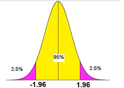
临界值:如下图所示,我们把左右两边的 2.5%
的面积定义为小概率事件,即紫色部分为小概率事件。这两个紫色区域的临界值的横坐标为:
Critical value: As shown in the figure below, we define the 2.5% area on both the left and right sides as a low-probability event, that is, the purple part is a low-probability event. The horizontal coordinates of the critical values of these two purple areas are:
那么如何计算一个样本的统计量呢?statsmodels.stats.weightstats
库中的
ztest
可以实现这个过程。
So how do you calculate the statistics of a sample? statsmodels.stats.weightstats
in the ztest library can accomplish this process.
ztest
函数包含的输入参数如下:
The input parameters included in the function are as follows:
x1:样本的数据值。 x1: The data value of the sample.
value:原假设中总体的均值。 value: The mean of the population in the null hypothesis.
该函数的原假设
The null hypothesis of the function
tstats:统计量值 tstats: statistical value
pvalue:p 值 p-value: p value
如果这里存在一个样本集合
arr,让我们通过假设检验推断一下该样本对应的总体的均值是否为
If there is a sample set arr, let's infer through hypothesis testing whether the mean of the population corresponding to this sample is
首先让我们来定义样本容量超过 30 的样本集合,因为只有超过 30
的样本集合的均值才能使用 z 检验进行推断。
First, let's define a sample set with a sample size greater than 30, because only the mean of a sample set with more than 30 samples can be inferred using the z-test.
arr = [23, 36, 42, 34, 39, 34, 35, 42, 53, 28, 49, 39, 46, 45, 39, 38, 45, 27,
       43, 54, 36, 34, 48, 36, 47, 44, 48, 45, 44, 33, 24, 40, 50, 32, 39, 31]
len(arr)
36
接下来,让我们使用
ztest
计算原假设所对应的统计量 z:
Next, let's use ztest to calculate the test statistic z corresponding to the null hypothesis:
import statsmodels.stats.weightstats as sw

# 原假设为总体的平均值是 39
z, p = sw.ztest(arr, value=39)
z
0.3859224924939799
从结果可以看到,原假设的统计量 z = 0.38,该值刚好大于
-1.96,小于 1.96。因此,我们应当接受原假设。
From the results, it can be seen that the test statistic for the null hypothesis is z = 0.38, which is just greater than -1.96 and less than 1.96. Therefore, we should accept the null hypothesis.
综上,我们可以得到样本所对应的总体的平均值等于 39。
In summary, we can conclude that the mean of the population corresponding to the sample is 39.
如果将原假设改为:样本所对应的总体的平均值为
20。让我们重新来计算统计量 t:
If the null hypothesis is changed to: the mean of the population corresponding to the sample is 20. Let's recalculate the t statistic:
z, p = sw.ztest(arr, value=20)
z
15.050977207265216
从结果可以看出,z 的值远远大于
1.96。因此,我们应当拒绝该假设,接受与之对应的备选假设,即总体的平均值不等于
20。
From the results, it can be seen that the value of z is much greater than 1.96. Therefore, we should reject the null hypothesis and accept the corresponding alternative hypothesis, which means that the population mean is not equal to 20.
当然,上面的 z 检验方案只是 z 检验的一种。我们还可以按照
{临界值只有左边存在、临界值只有右边存在、临界值两边都存在}
等三种可能,将 z 检验类型分为
{左侧检验、右侧检验和双侧检验}。
Of course, the above z-test scheme is just one type of z-test. We can also classify the z-test into three types: {left-tailed test, right-tailed test, and two-tailed test} based on the three possible scenarios: {critical value exists only on the left, critical value exists only on the right, and critical values exist on both sides}.
利用统计量判断原假设是否拒绝并不是唯一的方法,我们还可以使用
Using statistics to determine whether to reject the null hypothesis is not the only method; we can also use the
我们一般认为如果
We generally believe that if the
其实使用
In fact, using the
因此,大家都喜欢使用
Therefore, everyone prefers to use the
其实假设检验是统计学中最重要的一部分,它还包含了很多知识点。但是由于这些知识点在机器学习中使用并不频繁(数据分析中经常使用),就不做赘述了。
Actually, hypothesis testing is one of the most important parts of statistics, and it includes many knowledge points. However, since these knowledge points are not frequently used in machine learning (they are often used in data analysis), they will not be elaborated on.
90.17. 总结# 90.17. Summary #
本实验首先讲解了概率论中的三大公式,这个公式在朴素贝叶斯算法中使用频繁。然后,讲解了离散分布和连续型分布的具体区别,以及常用的分布函数式子和图像。最后对统计学中的假设检验进行了相关的讲解与实现。
This experiment first explained the three major formulas in probability theory, which are frequently used in the Naive Bayes algorithm. Then, it explained the specific differences between discrete and continuous distributions, as well as commonly used distribution functions and graphs. Finally, it provided relevant explanations and implementations of hypothesis testing in statistics.
○ 推荐安装
GetVM
浏览器扩展,使用其提供的
Jupyter Notebook
在线环境进行代码实践。
○ It is recommended to install the GetVM browser extension and use its provided Jupyter Notebook online environment for code practice.
○ 欢迎分享本文链接到你的社交账号、博客、论坛等。更多的外链会增加搜索引擎对本站收录的权重,从而让更多人看到这些内容。
○ Welcome to share this article link to your social accounts, blogs, forums, etc. More external links will increase the search engine's ranking of this site, allowing more people to see this content.