Trace comparisons arrive in Jaeger 1.7Jaeger 1.7 中提供了跟踪比较

Distributed tracing can capture a wealth of data and has the potential to yield invaluable insights. But, bridging the gap between the ocean of spans and the epiphanies they offer is not yet a solved problem.
分布式跟踪可以捕获大量数据，并有可能产生宝贵的见解。但是，弥合浩瀚的跨度与它们所提供的顿悟之间的差距还不是一个已解决的问题。

As of Jaeger 1.7, the ability to compare traces is now available in the Jaeger UI. We are hopeful trace comparisons will facilitate going from data to decisions.
从 Jaeger 1.7 开始，Jaeger UI 中现在提供了比较跟踪的功能。我们希望跟踪比较能够促进从数据到决策的转变。

Overview 概述

The trace comparison feature enables the structural aspects of two traces to be compared. Each trace is condensed into a tree of unique service / operation paths. Then, differences in the presence or prevalence of nodes in the trees are emphasized with color-coding. For instance, when comparing two traces which are essentially RPC call-graphs, the comparison highlights which call sequences are present in only one of the traces or occur more frequently in one of the traces.
迹线比较功能可以比较两条迹线的结构。每个跟踪都被压缩成一棵独特的服务/操作路径树。然后，通过颜色编码强调树中节点的存在或普遍性的差异。例如，当比较本质上是 RPC 调用图的两个跟踪时，比较会突出显示哪些调用序列仅出现在其中一个跟踪中，或者在其中一个跟踪中更频繁地出现。

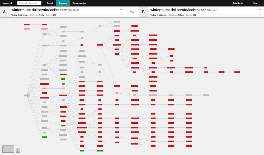
In the screenshot above, the dark red nodes are nodes which happened in trace A but do not exist in trace B. We can see very clearly that trace B is primarily a subset of trace A (more on that, below).
在上面的屏幕截图中，深红色节点是在迹线 A 中发生但在迹线 B 中不存在的节点。我们可以非常清楚地看到，迹线 B 主要是迹线 A 的子集（更多内容见下文）。

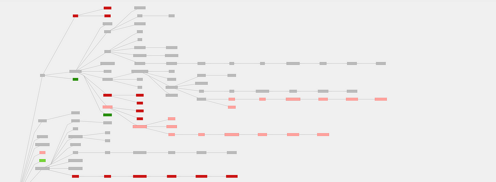
In addition to emphasizing spans which are present in only one of the traces, trace comparisons also indicate when spans are repeated more often in one trace or the other. For instance, in the comparison of two traces from the HotROD example, below, we can see the node for redis::GetDriver is light green and marked with +1 and +8%. This lets us know the span is present in both traces but it is seen more often in trace B.
除了强调仅在一条迹线中出现的跨度之外，迹线比较还指示跨度何时在一条迹线或另一条迹线中更频繁地重复。例如，在下面 HotROD 示例中两条迹线的比较中，我们可以看到 redis::GetDriver 的节点为浅绿色，并标记为 +1 和 +8% 。这让我们知道跨度存在于两条迹线中，但在迹线 B 中更常见。

The color-coding of the differences is inspired by code review tools. When comparing trace A to trace B, we evaluate the differences as if we wanted to change trace A to have the same structure as trace B: what would we need to remove from trace A or add to trace A in order to achieve an equivalent structure with trace B.
差异的颜色编码受到代码审查工具的启发。当比较迹线 A 和迹线 B 时，我们评估差异，就好像我们想要将迹线 A 更改为与迹线 B 具有相同的结构：我们需要从迹线 A 中删除什么或添加到迹线 A 中才能实现等效的结构与迹线 B.

Dark colors indicate the node is missing from one of the traces:
深色表示该节点在其中一条迹线中缺失：

• Dark red: The node is only in trace A and would need to be **removed** in order to match B
  深红色：该节点仅位于迹线 A 中，需要**删除**才能匹配 B
• Dark green: The node is only in trace B and would need to be **added** in order to match B
  深绿色：该节点仅位于迹线 B 中，需要**添加**才能匹配 B

Light colors indicate the node is present in both traces but more-so in one or the other:
浅色表示该节点存在于两条迹线中，但在其中一条迹线中更是如此：

• Light red: The node in A has more spans than B
  浅红色：A中的节点比B中的节点具有更多的跨度
• Light green: The node in B has more spans than A
  浅绿色：B 中的节点比 A 中的节点具有更多的跨度

Gray indicates the two traces both have that node and have the same number of spans grouped into it.
灰色表示两条迹线都具有该节点，并且分组到其中的跨度数量相同。

Now that we know what, how about why?
既然我们知道了什么，那为什么呢？

The pattern where one trace is a subset of another trace, and the missing portion is non-trivial, is typical when comparing a request which was processed successfully against a request which was interrupted by an error.
在将成功处理的请求与因错误中断的请求进行比较时，典型的模式是，一个跟踪是另一跟踪的子集，并且丢失的部分非常重要。

Such a comparison can offer a very timely and relevant insight when investigating an incident. We can quickly and confidently narrow our search space — sometimes to a much smaller area of interest.
在调查事件时，这种比较可以提供非常及时且相关的见解。我们可以快速、自信地缩小搜索空间——有时缩小到更小的感兴趣区域。

Assuming that our error trace is representative of the incident (and, ideally, we would have several traces to draw from), we can infer that investigating the red nodes is almost certainly not the best use of our time because they are not even visited in the error trace.
假设我们的错误跟踪代表了事件（并且，理想情况下，我们将有多个跟踪可供借鉴），我们可以推断，调查红色节点几乎肯定不是我们时间的最佳利用，因为它们甚至没有被访问过错误跟踪。

Meanwhile, it’s possible the red nodes represent a substantial number of monitored resources which, as part of the incident, may be experiencing a severe drop in load. Thus, the unvisited nodes just might be slamming us with alerts (relatively speaking). Under such circumstances, it’s not unfathomable to think: “OMG! These alerts are from services that aren’t even in the [error] traces we’re digging into! WTF! FML!” TLDR: Not good.
同时，红色节点可能代表大量受监控资源，作为事件的一部分，这些资源可能会经历负载严重下降。因此，未访问的节点可能会向我们发出警报（相对而言）。在这种情况下，不难想象：“天啊！这些警报来自的服务甚至不在我们正在挖掘的[错误]跟踪中！卧槽！卧槽！” TLDR：不好。

Ordinarily, focusing on the error trace(s) when we’re being barraged by alerts from disparate sources that aren’t present in our error traces requires two or more of the following traits:
通常，当我们受到错误跟踪中不存在的不同来源的警报的攻击时，专注于错误跟踪需要以下两个或多个特征：

• Nerves of adamantium 金刚烷神经
• A venerable lineage of prior incidents to draw from
  历史悠久的历史事件可供借鉴
• A zen-like relationship with entropy and adrenaline
  熵和肾上腺素的禅宗般的关系

Or, we can lean on our insights from the trace comparison to transcend the clamor.
或者，我们可以依靠痕迹比较的见解来超越喧嚣。

Disclaimer: My excitement for the trace comparison feature (and my penchant for drama) may have gotten the better of me, here. Please understand the above is a dramatic re-enactment of a hypothetical outage scenario.
免责声明：我对痕迹比较功能的兴奋（以及我对戏剧的偏好）可能已经战胜了我。请理解以上内容是假设的中断场景的戏剧性重演。

How? — Group, match and compare
如何？ — 分组、匹配和比较

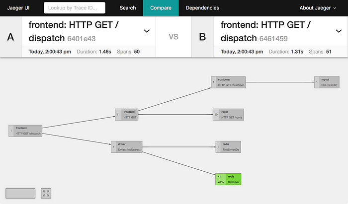
In the comparison of the HotROD traces above, you may have noticed there are far fewer nodes in the comparison graph than spans in the traces (8 vs 50).
在上面 HotROD 轨迹的比较中，您可能已经注意到比较图中的节点比轨迹中的跨度少得多（8 个与 50 个）。

The comparison feature first reduces a trace to a more compact graph representation. This is done by collecting spans into groups, and representing the trace as a DAG (directed acyclic graph) of these groups instead of as a DAG of individual spans. Then, it’s these groups of spans which are matched between traces and compared.
比较功能首先将迹线减少为更紧凑的图形表示。这是通过将跨度收集到组中并将迹线表示为这些组的 DAG（有向无环图）而不是单个跨度的 DAG 来完成的。然后，这些跨度组在迹线之间进行匹配和比较。

Why collect spans into groups?
为什么将跨度收集到组中？

In our experience, grouping “similar” spans facilitates analysis by making trace comparisons more comprehensible, in some cases dramatically so.
根据我们的经验，对“相似”跨度进行分组可以使跟踪比较更容易理解，在某些情况下甚至更容易理解，从而促进分析。

As a baseline, if we were to compare two traces in their raw form, our comparison would be based on spans being common to both traces or being only in trace A or only in trace B.
作为基线，如果我们要比较原始形式的两条迹线，我们的比较将基于两条迹线共有的跨度或仅在迹线 A 中或仅在迹线 B 中。

Where does that leave us? Let’s take a look at three traces, each rooted at ROOT_SVC.
那我们会怎样呢？让我们看一下三个跟踪，每个跟踪都以 ROOT_SVC 为根。

Trace Alpha has one child span:
Trace Alpha 有一个子跨度：

ROOT_SVC – CHILD_SVC

Trace Beta has a root span with three children:
Trace Beta 的根跨度包含三个子节点：

         CHILD_SVC
        /  
ROOT_SVC – CHILD_SVC
        \  
         CHILD_SVC

Trace Gamma also has a root spans with three children:
Trace Gamma 也有一个包含三个子项的根跨度：

         CHILD_SVC
        /  
ROOT_SVC – ANOTHER_CHILD_SVC
        \  
         A_THIRD_CHILD_SVC

With our baseline comparison, comparing Alpha vs Beta and comparing Alpha vs Gamma would result in a graph where ROOT_SVC has a gray child-node for the CHILD_SVC span shared between the two traces and two dark green nodes indicating those spans are not in trace A.
通过我们的基线比较，比较 Alpha 与 Beta 以及比较 Alpha 与 Gamma 将得到一个图表，其中 ROOT_SVC 对于两条迹线之间共享的 CHILD_SVC 范围有一个灰色子节点，并且两个深绿色节点指示这些范围不在迹线 A 中。

Naturally, there is validity to this result, but it can be very verbose and does not indicate Alpha and Beta actually have a lot more in common than Alpha and Gamma. We can do better.
当然，这个结果是有效的，但它可能非常冗长，并且并不表明 Alpha 和 Beta 实际上比 Alpha 和 Gamma 有更多的共同点。我们可以做得更好。

The three CHILD_SVC nodes in trace Beta do have common ground: They represent the same logical element (CHILD_SVC, in our example) and they have the same parent. We can leverage this by collecting the three CHILD_SVC spans in trace Beta into a group. The impact of this grouping is two-fold:
跟踪 Beta 中的三个 CHILD_SVC 节点确实有共同点：它们代表相同的逻辑元素（在我们的示例中为 CHILD_SVC）并且具有相同的父节点。我们可以通过将跟踪 Beta 中的三个 CHILD_SVC 范围收集到一个组中来利用这一点。这种分组的影响有两个方面：

• It allows us to simplify our representation of the comparison
  它使我们能够简化比较的表示
• It visually encodes the similarity of spans by grouping them
  它通过对跨度进行分组来直观地编码跨度的相似性

When we apply this grouping to the Alpha vs Beta comparison, we end up with a single child which we color light green to indicate the node has a heavier presence in Beta than Alpha. Our decision to group nodes has no impact on the Alpha vs Gamma comparison.
当我们将此分组应用于 Alpha 与 Beta 比较时，我们最终得到一个子节点，我们将其着色为浅绿色，以表明该节点在 Beta 中的存在比 Alpha 中的存在更重。我们对节点进行分组的决定对 Alpha 与 Gamma 比较没有影响。

The new representation of Alpha vs Beta ends up being much simpler than the Alpha vs Gamma comparison, which makes intuitive sense because Gamma is a more diverse set of nodes than either Alpha or Beta.
Alpha 与 Beta 的新表示最终比 Alpha 与 Gamma 的比较简单得多，这具有直观意义，因为 Gamma 是比 Alpha 或 Beta 更多样化的节点集。

Our definition of “similar”
我们对“相似”的定义

We define two spans to be similar, which is to say we put them in the same group, if and only if:
我们将两个跨度定义为相似的，也就是说，我们将它们放在同一组中，当且仅当：

• They have the same ordered set of ancestors as defined by the service and operation of the ancestors
  它们具有由祖先的服务和操作定义的相同的有序祖先集
• They are both either parents or leaves
  他们要么是父母，要么是叶子

For example: 例如：

         CHILD_SVC
        /  
ROOT_SVC – CHILD_SVC
        \  
         CHILD_SVC

Would reduce to the following, with the (3) indicating the CHILD_SVC node is a group of three spans:
将减少为以下内容，其中 (3) 指示 CHILD_SVC 节点是一组三个跨度：

ROOT_SVC – CHILD_SVC (3)

And, the following trace would not reduce at all:
并且，以下痕迹根本不会减少：

         CHILD_SVC
        /  
ROOT_SVC – CHILD_SVC – CHILD_SVC
        \  
         ANOTHER_CHILD_SVC

While this definition of “similar” has both pros and cons, and is essentially arbitrary, we have found it to be very practical.
虽然“相似”的这个定义有利有弊，而且本质上是任意的，但我们发现它非常实用。

Comparing groups 比较组

Our baseline comparison allowed us to compare traces based only on whether a span is “present” or “absent.” That’s to say, whether a span should be inserted into trace A or removed from trace B to achieve an equivalent structure between the two traces. We can continue to apply this relationship if we apply it to groups of spans instead of individual spans.
我们的基线比较使我们能够仅根据跨度是“存在”还是“不存在”来比较迹线。也就是说，是否应该在迹线 A 中插入一个跨度，或者从迹线 B 中删除一个跨度，以实现两条迹线之间的等效结构。如果我们将其应用于跨度组而不是单个跨度，我们可以继续应用这种关系。

Further, when a group of spans is present in both traces, we can compare the number of spans in each trace’s group.
此外，当两个迹线中都存在一组跨度时，我们可以比较每个迹线组中的跨度数量。

Trace comparisons are now a collection of the following relationships between groups of spans:
跟踪比较现在是跨度组之间以下关系的集合：

• The group is only in trace A (dark red)
  该组仅存在于迹线 A（深红色）中
• The group is only in trace B (dark green)
  该组仅位于迹线 B 中（深绿色）
• The group is in both traces but has more spans in trace A (light red)
  该组位于两条迹线中，但在迹线 A 中具有更多跨度（浅红色）
• The group is in both traces but has more spans in trace B (light green)
  该组位于两条迹线中，但在迹线 B 中具有更多跨度（浅绿色）
• The group is in both traces and contains the same number of spans (gray)
  该组位于两条迹线中并且包含相同数量的跨度（灰色）

Future work 未来的工作

We are interested in the following enhancements:
我们对以下增强功能感兴趣：

• Comparison of span attributes , such as the average duration of spans in a group, rather than the number of spans in the group
  Span属性的比较，例如组中Span的平均持续时间，而不是组中Span的数量
• Introducing the ability to adjust the coarseness of how groups are establish — see jaeger-ui#252
  引入了调整组建立方式粗细度的功能 - 请参阅 jaeger-ui#252