Bayesian Modeling of Biomolecular Assemblies with Cryo-EM Maps使用冷冻电镜图谱对生物分子组装进行贝叶斯建模

A growing array of experimental techniques allows us to characterize the three-dimensional structure of large biological assemblies at increasingly higher resolution. In addition to X-ray crystallography and nuclear magnetic resonance in solution, new structure determination methods such cryo-electron microscopy (cryo-EM), crosslinking/mass spectrometry and solid-state NMR have emerged. Often it is not sufficient to use a single experimental method, but complementary data need to be collected by using multiple techniques. The integration of all datasets can only be achieved by computational means. This article describes Inferential structure determination, a Bayesian approach to integrative modeling of biomolecular complexes with hybrid structural data. I will introduce probabilistic models for cryo-EM maps and outline Markov chain Monte Carlo algorithms for sampling model structures from the posterior distribution. I will focus on rigid and flexible modeling with cryo-EM data and discuss some of the computational challenges of Bayesian inference in the context of biomolecular modeling.
越来越多的实验技术使我们能够以越来越高的分辨率表征大型生物组装的三维结构。除了 X 射线晶体学和溶液核磁共振外，新的结构测定方法如冷冻电子显微镜（cryo-EM）、交联/质谱和固态 NMR 已经出现。通常，仅使用单一实验方法是不够的，但需要通过使用多种技术收集互补数据。所有数据集的整合只能通过计算手段实现。本文描述了推断结构测定，这是一种贝叶斯方法，用于整合具有混合结构数据的生物分子复合物的建模。我将介绍用于 cryo-EM 图的概率模型，并概述从后验分布中抽样模型结构的马尔可夫链蒙特卡洛算法。我将重点介绍使用 cryo-EM 数据进行刚性和柔性建模，并讨论在生物分子建模背景下贝叶斯推断的一些计算挑战。

1. Introduction  1. 引言

Thanks to groundbreaking advances in experimental techniques it has become possible to study the structure of large biological assemblies at increasingly higher resolution. Traditionally, high-resolution biomolecular structure determination was only possible by X-ray crystallography or nuclear magnetic resonance (NMR) in solution (Berman et al., 2000). The application of NMR and X-ray crystallography to larger systems remained challenging due to the sheer size of the system and/or because it was difficult to find suitable crystallization conditions. More recently, emerging methods such as cryo-electron microscopy (cryo-EM) (Frank, 2002; Orlova and Saibil, 2004; Chiu et al., 2005), crosslinking/mass spectrometry (Gingras et al., 2007; Rappsilber, 2011) and solid-state NMR (Yan et al., 2013) have started to provide exciting insights into the structure of large macromolecular assemblies that was previously very difficult, if not impossible to obtain. In particular, cryo-EM has reached near-atomic and in some cases even atomic resolution over the last 5 years (Bai et al., 2015; Fischer et al., 2015; Khatter et al., 2015). The EM databank (EMDB) (Lawson et al., 2011) stores an increasing number of high-resolution EM reconstructions. Several biologically essential assemblies that resisted high-resolution studies have recently been characterized by cryo-EM including spliceosomal complexes (Yan et al., 2015; Agafonov et al., 2016; Galej et al., 2016; Rauhut et al., 2016; Wan et al., 2016), eukaryotic ribosomes (Anger et al., 2013; Khatter et al., 2015), and transcription initiation complexes (Plaschka et al., 2015).
由于实验技术的突破性进展，已经有可能以越来越高的分辨率研究大型生物组装的结构。传统上，高分辨率的生物大分子结构测定只能通过 X 射线晶体学或溶液中的核磁共振（NMR）来实现（Berman 等人，2000 年）。由于系统的庞大尺寸和/或难以找到合适的结晶条件，将 NMR 和 X 射线晶体学应用于更大系统一直具有挑战性。最近，新兴方法如冷冻电子显微镜（cryo-EM）（Frank，2002 年；Orlova 和 Saibil，2004 年；Chiu 等人，2005 年）、交联/质谱（Gingras 等人，2007 年；Rappsilber，2011 年）和固态 NMR（Yan 等人，2013 年）已经开始提供关于大型大分子组装结构的令人兴奋的见解，这些结构以前很难获得，如果不是不可能的话。特别是，在过去 5 年中，冷冻电子显微镜已经达到了近原子甚至原子分辨率（Bai 等人，2015 年；Fischer 等人，2015 年；Khatter 等人，2015 年）。 EM 数据库（EMDB）（Lawson 等人，2011 年）存储了越来越多的高分辨率电子显微重建图。最近，包括剪接体复合物（Yan 等人，2015 年；Agafonov 等人，2016 年；Galej 等人，2016 年；Rauhut 等人，2016 年；Wan 等人，2016 年）、真核生物核糖体（Anger 等人，2013 年；Khatter 等人，2015 年）和转录起始复合物（Plaschka 等人，2015 年）在内的几个生物学上至关重要的复合物通过冷冻电子显微镜得到了表征。

Although several powerful experimental techniques are available that allow us to study the structure of large biomolecular systems, we need computational methods that assist us in integrative modeling with diverse structural data (Sali et al., 2003; Robinson et al., 2007; Ward et al., 2013). The reasons for developing new computational methods are both of a principled and practical nature.
尽管我们有几种强大的实验技术可以用来研究大型生物分子系统的结构，但我们仍需要计算方法来协助我们整合来自不同结构数据（Sali 等人，2003 年；Robinson 等人，2007 年；Ward 等人，2013 年）的综合建模。开发新的计算方法的原因是原则性和实用性的。

Structural models built from hybrid data should be as objective as possible and ideally not be biased by a human modeler, therefore automated computational modeling tools are indispensable (Karaca and Bonvin, 2013; Villa and Lasker, 2014; Schröder, 2015). The models should be compatible with all of the available data, which might come from different experimental sources. The modeling software should also be able to integrate data-independent prior information about the system.
从混合数据构建的结构模型应尽可能客观，理想情况下不应受到人类建模者的偏见影响，因此自动计算建模工具是必不可少的（Karaca 和 Bonvin，2013；Villa 和 Lasker，2014；Schröder，2015）。模型应与所有可用的数据兼容，这些数据可能来自不同的实验来源。建模软件还应能够整合关于系统的与数据无关的先验信息。

Most existing refinement and modeling software focuses on structural data of a particular type. For example, a number of software packages for X-ray structure refinement or modeling with NMR restraints exist. To use these packages for modeling with hybrid data is often difficult and involves some sort of tweaking. We therefore need a versatile software that can integrate diverse types of structural information (Russel et al., 2012).
大多数现有的精修和建模软件都专注于特定类型的结构数据。例如，存在许多用于 X 射线结构精修或使用 NMR 限制进行建模的软件包。使用这些软件包进行混合数据建模通常很困难，并且涉及某种调整。因此，我们需要一个能够整合多种类型结构信息的多功能软件（Russel 等人，2012）。

Every software for integrative modeling with hybrid data has to address the following questions: How much weight should the various pieces of information be given? How to deal with datasets that (partially) contradict some of the other datasets? Obviously, the weights can have a strong impact on the final structure (Brünger, 1992; Habeck et al., 2006), and it would be desirable to choose the weights in a data-driven, self-adaptive fashion. Because the individual datasets themselves typically provide only ambiguous structural information, we have to fit the model against all data simultaneously to obtain the least ambiguous result. What is a good representation of the remaining uncertainty about the structure? We need to represent the ambiguity of the structural model adequately.
每个用于混合数据综合建模的软件都必须解决以下问题：应该如何赋予各种信息不同的权重？如何处理与其他数据集（部分）矛盾的数据集？显然，权重对最终结构可能有很大影响（Brünger, 1992; Habeck et al., 2006），因此希望以数据驱动、自适应的方式选择权重。由于单个数据集本身通常只提供模糊的结构信息，我们必须同时拟合所有数据以获得最不模糊的结果。关于结构的剩余不确定性有什么好的表示方法？我们需要充分表示结构模型的不确定性。

The software should also be able to integrate data of varying resolution. A common scenario is that high-resolution information about the subunits in isolation is available (Esquivel-Rodríguez and Kihara, 2013), such that modeling the complex appears to be simple: we just need to put the pieces together. However, even in this seemingly simple situation several issues need to be considered.
软件还应能够整合不同分辨率的数据。一个常见的情况是，关于孤立亚基的高分辨率信息是可用的（Esquivel-Rodríguez 和 Kihara，2013），因此对复合物进行建模似乎很简单：我们只需要把各部分拼凑在一起。然而，即使在这种看似简单的情况下，也需要考虑几个问题。

The formation of the complex is often accompanied by a conformational change in the subunits (Gerstein et al., 1994). How much should we deviate from the known structures of the free subunits in order to fit the data of the complex? If the data is sparse (e.g., crosslinking or NMR data) or of a medium resolution, there is the risk of overfitting the data.
复合物的形成通常伴随着亚基构象的变化（Gerstein 等人，1994 年）。我们应该偏离已知自由亚基结构的程度是多少才能适应复合物的数据？如果数据稀疏（例如，交联或 NMR 数据）或分辨率中等，则存在过度拟合数据的风险。

Another practical problem is the enormous size of the systems that can comprise tens of thousands up to millions of atoms. Is there enough information to determine the position of all atoms? Or should we rather lower our goal and aim for a coarse-grained, intermediate resolution model?
另一个实际问题是系统的巨大规模，可能包含数万到数百万个原子。是否有足够的信息来确定所有原子的位置？或者我们应该降低目标，追求一个粗粒度的中等分辨率模型？

At the source of many of these issues is the question of how to deal with uncertainty in the data and about our model. We need a mathematical framework to quantitatively represent any uncertainty in the process that takes us from the input data to the final model. The framework should allow us to follow the propagation of the uncertainty about a biomolecular structure as we combine data from diverse sources and to compute structural error bars that reflect the degree of uncertainty.
在许多这些问题的源头是关于如何处理数据中的不确定性以及我们模型的问题。我们需要一个数学框架来定量表示从输入数据到最终模型的过程中存在的任何不确定性。该框架应允许我们跟踪随着我们从不同来源合并数据时关于生物分子结构的不确定性的传播，并计算反映不确定性程度的结构误差范围。

Bayesian probability theory is a unique and objective mathematical framework for quantitative inference from limited, diverse and uncertain information (Cox, 1946; Jaynes, 2003; MacKay, 2003). The essence of the Bayesian approach is that any probability should be interpreted as incomplete information about a quantity rather than a frequency of occurrence. Highly ambiguous and uncertain information results in multi-modal distributions that are spread out over many parameter values. Markov chain Monte Carlo (MCMC) methods (Liu, 2001) allow us to apply the Bayesian formalism in practice even to highly complex data and models.
贝叶斯概率论是一种独特且客观的数学框架，用于从有限、多样化和不确定的信息中进行定量推断（Cox，1946；Jaynes，2003；MacKay，2003）。贝叶斯方法的核心是任何概率都应该被解释为关于一个量的不完整信息，而不是发生的频率。高度模糊和不确定的信息导致多模态分布，这些分布在许多参数值上展开。马尔可夫链蒙特卡洛（MCMC）方法（Liu，2001）允许我们在实践中应用贝叶斯形式主义，即使是对于高度复杂的数据和模型。

More than a decade ago, Bayesian methods have been introduced for protein structure determination from solution NMR data (Rieping et al., 2005; Habeck, 2012). In this article, I will describe recent developments in Bayesian integrative modeling with hybrid data.
十多年前，贝叶斯方法已被引入用于从溶液 NMR 数据确定蛋白质结构（Rieping 等人，2005 年；Habeck，2012 年）。在本文中，我将描述贝叶斯综合建模与混合数据的最新发展。

2. Methods  2. 方法

2.1. Inferential Structure Determination
2.1 推理结构确定

Inferential structure determination (ISD) is the first strictly statistical approach to biomolecular modeling (Habeck et al., 2005a; Rieping et al., 2005). Originally ISD was developed for solution NMR data on small protein domains (Rieping et al., 2008; Habeck, 2012). But the basic principle can be applied to large systems and diverse structural data (Bayrhuber et al., 2008; Shahid et al., 2012; Habenstein et al., 2015).
推断结构确定（ISD）是第一个严格的生物分子建模统计方法（Habeck 等人，2005a；Rieping 等人，2005）。最初 ISD 是为了解决小蛋白质域的溶液 NMR 数据而开发的（Rieping 等人，2008；Habeck，2012）。但基本原理可以应用于大型系统和多样化的结构数据（Bayrhuber 等人，2008；Shahid 等人，2012；Habenstein 等人，2015）。

At the core of the ISD approach is a probabilistic formulation of the structure determination problem. We have to distinguish two principal types of information that guide us in the modeling of a biomolecular structure: the experimental data D and data-independent prior information I about biomolecular structures. All the information is encoded statistically through conditional probabilities. The probability:
ISD 方法的核心是结构确定问题的概率表述。我们必须区分两种主要类型的信息，这些信息在生物分子结构的建模中指导我们：实验数据 D 和关于生物分子结构的数据独立先验信息 I。所有信息都通过条件概率统计编码。概率：

$\mathrm{Pr}\left(D\right|\theta ,I)$

quantifies how probable it is to observe data D if the actual configuration of the system is θ. Pr(D|θ, I) is called the likelihood function. The prior probability:
量化在系统实际配置为θ的情况下观察到数据 D 的可能性。Pr(D|θ, I)被称为似然函数。先验概率：

$\mathrm{Pr}\left(\theta \right|I)$

expresses what we know about reasonable system configurations θ without observing any data.
表达了我们在没有观察任何数据的情况下对合理系统配置θ的了解。

Probability calculus allows us to combine both types of information and to derive a posterior distribution over all conformational degrees of freedom by invoking Bayes' theorem (Jaynes, 2003):
概率演算允许我们结合这两种类型的信息，并通过调用贝叶斯定理（Jaynes，2003）推导出所有构象自由度的后验分布

$\mathrm{Pr}\left(\theta \right|D,I)=\frac{1}{\mathrm{Pr}\left(D\right|I)}\mathrm{Pr}(D|\theta ,I)\mathrm{Pr}\left(\theta \right|I).$

The posterior Pr(θ|D, I) expresses what we know about the unknown structure given the experimental data D and our prior knowledge I. The probability Pr(D|I) (the so-called model evidence) can be ignored if we are only interested in estimating θ, because Pr(D|I) does not depend on θ. However, if we aim to compare different prior or modeling assumptions, it will be important to calculate Pr(D|I) (Habeck, 2011; Mechelke and Habeck, 2012, 2014; Knuth et al., 2015).
后验概率 Pr(θ|D, I)表达了我们在给定实验数据 D 和先验知识 I 的情况下对未知结构的了解。如果我们只对估计θ感兴趣，可以忽略概率 Pr(D|I)（所谓的模型证据），因为 Pr(D|I)不依赖于θ。然而，如果我们旨在比较不同的先验或建模假设，计算 Pr(D|I)将会很重要（Habeck, 2011; Mechelke 和 Habeck, 2012, 2014; Knuth 等人, 2015）。

Often, we need to introduce additional unknown parameters to express our prior information or to model the experimental data. Let's denote these parameters by ξ; in statistical parlance, ξ are nuisance parameters. It is straightforward to infer both θ and ξ from the experimental data. All we need to do is to introduce a prior probability for the model parameters ξ and to invoke Bayes' theorem on the joint parameter space:
通常，我们需要引入额外的未知参数来表达我们的先验信息或对实验数据进行建模。让我们用ξ表示这些参数；在统计术语中，ξ是干扰参数。从实验数据中推断θ和ξ是直接的。我们所需要做的就是为模型参数ξ引入一个先验概率，并在联合参数空间上调用贝叶斯定理：

$\mathrm{Pr}(\theta ,\xi |D,I)=\frac{1}{\mathrm{Pr}\left(D\right|I)}\mathrm{Pr}(D|\theta ,\xi ,I)\mathrm{Pr}\left(\theta \right|I\left)\mathrm{Pr}\right(\xi \left|I\right).$

where we assumed that θ and ξ are independent a priori: Pr(θ, ξ|I) = Pr(θ|I) Pr(ξ|I). It is straightforward to relax this assumption if necessary.
我们假设θ和ξ事先是独立的：Pr(θ, ξ|I) = Pr(θ|I) Pr(ξ|I)。如果有必要，放宽这个假设是直接的。

The posterior probability Pr(θ, ξ|D, I) encodes all available information about the unknown parameters. In biomolecular structure determination, the posterior is typically too complex to do any further analytical calculations. By drawing Monte Carlo samples from Pr(θ, ξ|D, I) we generate a finite approximation of the posterior (Liu, 2001). These samples can be used to compute expectations and variances over the unknown parameters and thereby estimate the parameters and compute error bars.
后验概率 Pr(θ, ξ|D, I)编码了关于未知参数的所有可用信息。在生物分子结构测定中，后验通常过于复杂，无法进行进一步的分析计算。通过从 Pr(θ, ξ|D, I)中抽取蒙特卡洛样本，我们生成了后验的有限近似（Liu, 2001）。这些样本可用于计算未知参数的期望和方差，从而估计参数并计算误差范围。

2.2. Probabilistic Models for Hybrid Data
2.2. 混合数据的概率模型

Before we can launch an ISD calculation, we need to choose a likelihood Pr(D|θ, ξ, I) and the priors Pr(θ|I) and Pr(ξ|I). The application of ISD to multiple datasets D_i is straightforward: Pr(D|θ, ξ, I) = ∏_i Pr(D_i|θ, ξ). Each dataset is described independently with an appropriate probabilistic model; all datasets are integrated by simply multiplying all factors representing the various datasets. Because probabilities for different datasets are calibrated (they all normalize to one), there is no issue of weighing the different datasets relative to each other.
在我们能够启动 ISD 计算之前，我们需要选择一个似然 Pr(D|θ, ξ, I)和先验 Pr(θ|I)和 Pr(ξ|I)。将 ISD 应用于多个数据集 D 是直接的：Pr(D|θ, ξ, I) = ∏ Pr(D|θ, ξ)。每个数据集都用一个适当的概率模型独立描述；通过简单地乘以代表各个数据集的所有因子来整合所有数据集。因为不同数据集的概率是校准的（它们都归一化为一），所以不存在相对权衡不同数据集的问题。

We use a Boltzmann distribution as a prior over the conformational degrees of freedom:
我们使用玻尔兹曼分布作为构象自由度的先验：

$\mathrm{Pr}\left(\theta \right|I)=\frac{1}{Z}\exp \{-E\left(\theta \right)\}\left(1\right)$

where E(θ) is a force field. ISD currently supports two force fields: a quartic repulsion term that lacks any attractive interaction, and a linearly ramped Lennard-Jones potential (see Habeck, 2011; Mechelke and Habeck, 2012 for more details). The prior distribution Pr(θ|I) allows us to restrict the conformational degrees of freedom such that reasonable model structures are preferred (for example, structures that are free of atom-atom clashes and have well-packed interfaces). The prior distribution over the model parameters Pr(ξ|I) is typically of a standard form and chosen such that sampling with MCMC is straightforward.
其中 E(θ)是一个力场。ISD 目前支持两种力场：一个缺乏任何吸引相互作用的四次排斥项，以及一个线性递减的 Lennard-Jones 势（更多细节见 Habeck, 2011; Mechelke 和 Habeck, 2012）。先验分布 Pr(θ|I)允许我们限制构象自由度，以便优先选择合理的模型结构（例如，没有原子间冲突且界面紧密堆积的结构）。模型参数的先验分布 Pr(ξ|I)通常是标准形式，并选择使得使用 MCMC 采样变得直接。

2.2.1. Probabilistic Model for EM Maps
2.2.1. EM 图的概率模型

The result of a cryo-EM study is a 3D reconstruction of the structure, which typically comes in the form of a regular cubic grid with equal grid spacing in all three spatial directions. To construct a probabilistic model for 3D reconstructions, we first need a mathematical relation that allows us to compute a theoretical density map from a given structure θ. ISD's current model for density maps is quite simple. The theoretical map is obtained from an atomic model by placing spherical Gaussians of the same size and weight at each atom. The theoretical density at 3D position x is:
冷冻电镜研究的结果是对结构的 3D 重建，通常以所有三个空间方向上等间距的规则立方网格形式出现。为了构建 3D 重建的概率模型，我们首先需要一个数学关系，允许我们从给定的结构θ计算理论密度图。ISD 当前对密度图的模型相当简单。理论图是通过在每个原子上放置相同大小和权重的球形高斯函数从原子模型获得的。3D 位置 x 处的理论密度是：

$\rho (x;\theta ,\sigma )=\sum _k\frac{1}{{\left(2\pi {\sigma }^2\right)}^{3/2}}\exp \{-\frac{1}{2{\sigma }^2}\parallel x-x_k(\theta \left){\parallel }^2\right\}\left(2\right)$

where the index k runs over all atoms that contribute to the density and x_k(θ) is the 3D position of the k-th atom in the structure parameterized by the conformational degrees of freedom θ. The theoretical density map can be interpreted as a blurred version of an atomic map with infinite resolution:
其中索引 k 遍历所有对密度有贡献的原子，x _k (θ)是由构象自由度θ参数化的结构中第 k 个原子的三维位置。理论密度图可以解释为具有无限分辨率的原子图的模糊版本：

$\rho (x;\theta ,\sigma )=g_{\sigma }*\rho (x;\theta ,0)\text{with}\rho (x;\theta ,0)=\sum _k\delta [x-x_k(\theta \left)\right]$

where δ is the Dirac delta function, g_σ is a Gaussian blur kernel with bandwidth σ and * denotes a 3D convolution. Model (2) is admittedly simplistic and valid only for modeling protein complexes at intermediate to low resolutions. For high-resolution maps and/or the modeling of protein/nucleic acid complexes the model should also incorporate atom-wise weights (proportional to atom mass) as well as scattering and temperature factors.
其中δ是狄拉克δ函数，g _σ 是具有带宽σ的高斯模糊核，*表示 3D 卷积。模型（2）无疑是简化的，仅适用于中等至低分辨率下蛋白质复合物的建模。对于高分辨率图谱和/或蛋白质/核酸复合物的建模，模型还应包含原子级权重（与原子质量成正比）以及散射和温度因子。

Let us assume that experimental values ρ_n are available at positions x_n (n = 1, …, N) which are typically the centers of voxels that make up a cubic grid. The discrepancy between the experimental map ρ_n and the theoretical map ρ(x_n; θ, σ) can be assessed with a Gaussian distribution. Alternative error models for density maps have been proposed (Vasishtan and Topf, 2011), but the Gaussian model is still the most widely used model.
假设在位置 x _n （n = 1, …, N）处可以获得实验值ρ _n ，这些位置通常是构成立方网格的体素的中心。实验图谱ρ _n 与理论图谱ρ(x _n ; θ, σ)之间的差异可以用高斯分布来评估。已经提出了密度图的其他误差模型（Vasishtan 和 Topf，2011），但高斯模型仍然是使用最广泛的模型。

The likelihood function resulting from a Gaussian model is:
由高斯模型得到的似然函数是：

$\begin{array}{c}\mathrm{Pr}\left(\rho \right|\theta ,\xi ,I)=\prod _{n=1}^N{\left(\frac{\lambda }{2\pi }\right)}^{1/2}\exp \left\{-\frac{\lambda }{2}{[{\rho }_n-\alpha \rho (x_n;\theta ,\sigma \left)\right]}^2\right\}\\ ={\left(\frac{\lambda }{2\pi }\right)}^{N/2}\exp \left\{-\frac{\lambda }{2}\sum _n{[{\rho }_n-\alpha \rho (x_n;\theta ,\sigma \left)\right]}^2\right\}& \left(3\right)\end{array}$

where the calibration factor α was introduced. There are three nuisance parameters ξ = (σ, α, λ). Typically, the bandwidth of the blur kernel σ is set to a constant value which depends on the resolution of the map. For example, the default value in Chimera (Pettersen et al., 2004) is σ = 0.225 × resolution. For this fixed choice of the bandwidth, σ can be absorbed into the background information I. However, it is also possible to estimate σ along with the other nuisance parameters and the conformational degrees of freedom.
其中引入了校准因子α。有三个干扰参数ξ = (σ, α, λ)。通常，模糊核的带宽σ被设置为一个取决于地图分辨率的常数值。例如，Chimera 中的默认值（Pettersen 等人，2004 年）是σ = 0.225 × 分辨率。对于这个固定的带宽选择，σ可以被吸收进背景信息 I 中。然而，也可以与其他干扰参数和构象自由度一起估计σ。

To estimate the scaling parameter, we have to look at the conditional posterior distribution:
为了估计缩放参数，我们必须查看条件后验分布：

$\begin{array}{c}\mathrm{Pr}\left(\alpha \right|\lambda ,\theta ,D,I)\propto \mathrm{Pr}(\alpha \left|I\right)\times \exp \{-\frac{\lambda \Vert \rho (\theta ,\sigma ){\Vert }^2}{2}\\ {\left(\alpha -\frac{{\sum }_n{\rho }_n\rho (x_n;\theta ,\sigma )}{\Vert \rho (\theta ,\sigma ){\Vert }^2}\right)}^2\}\end{array}$

where $\left|\right|\rho \left|\right|=\sqrt{{\sum }_n{\rho }_n^2}$. The second factor is a Gaussian centered about the estimator:
其中 $\left|\right|\rho \left|\right|=\sqrt{{\sum }_n{\rho }_n^2}$ 。第二个因素是以估计量为中心的高斯分布：

$\hat{\alpha }(\theta ,\sigma )=\frac{{\sum }_n{\rho }_n\rho (x_n;\theta ,\sigma )}{\Vert \rho (\theta ,\sigma ){\Vert }^2}\left(4\right)$

which is the slope of a straight line relating the calculated volume ρ(x_n; θ, σ) to the observed density ρ_n.
这是计算体积ρ(x _n ;θ,σ)与观测密度ρ _n 之间关系的直线的斜率。

The Gaussian model is directly related to the cross-correlation coefficient, which is often used to compare EM maps. To see this, let's integrate out the unknown scaling factor α. If we ignore the fact that α should be positive and choose a uniform (improper) prior over α (i.e., Pr(α|I) = const), we can analytically integrate out α to obtain a new likelihood that no longer depends on α (this procedure is also called marginalization in Bayesian statistics, Habeck et al., 2005a):
高斯模型直接与互相关系数相关，后者常用于比较 EM 图。为了看到这一点，让我们积分掉未知的缩放因子α。如果我们忽略α应该是正的事实，并选择在α上的均匀（不适当的）先验（即 Pr(α|I) = const），我们可以解析地积分掉α以获得一个新的似然，该似然不再依赖于α（这个过程在贝叶斯统计中也称为边缘化，Habeck 等人，2005a）：

$\begin{array}{c}\mathrm{Pr}\left(\rho \right|\theta ,\lambda ,I)=\int \text{d}\alpha \mathrm{Pr}(\rho |\theta ,\alpha ,\lambda ,I)\mathrm{Pr}\left(\alpha \right|I)\propto {\lambda }^{(N-1)/2}\\ \exp \{-\frac{\lambda \Vert \rho {\Vert }^2}{2}[1-C^2\left(\theta \right)\left]\right\}& \left(5\right)\end{array}$

where  在哪里

$C\left(\theta \right)=\frac{{\sum }_n{\rho }_n\rho (x_n;\theta ,\sigma )}{\parallel \rho \parallel \parallel \rho (\theta ,\sigma )\parallel }$

is the cross-correlation between the experimental and the theoretical map. The effective likelihood function (Equation 5) attains its maximum when the cross-correlation coefficient is one. Whenever we assess the goodness of fit between the model and the experimental map by means of the cross-correlation coefficient, we implicitly assume that the error of the EM map follows a Gaussian distribution.
是实验图和理论图之间的互相关。有效似然函数（方程 5）在互相关系数为一时达到最大值。每当我们通过互相关系数来评估模型与实验图之间的拟合优度时，我们隐含地假设 EM 图的误差遵循高斯分布。

The parameter λ is the inverse variance of the Gaussian likelihood (Equation 3) and called the precision of the model (Bernardo and Smith, 2009). It is also possible to estimate the precision λ of the fit between the experimental and the theoretical density map. The parameter λ assesses how well the experimental and theoretical map agree on average. For large λ, the experimental map is very reliable and imposes a strong force on the model to adapt itself such that the calculated map reproduces the observed map as closely as possible. Assuming Jeffreys's prior for the precision, i.e., Pr(λ|I) = 1/λ, the conditional posterior of the precision is a Gamma distribution (Habeck et al., 2006):
参数λ是高斯似然（方程 3）的方差的倒数，称为模型的精度（Bernardo 和 Smith，2009）。也可以估计实验密度图与理论密度图之间拟合的精度λ。参数λ评估实验图和理论图平均上的一致性如何。对于大的λ，实验图非常可靠，并对模型施加强大的力量使其适应，以便计算出的图尽可能地再现观测图。假设精度的 Jeffreys 先验，即 Pr(λ|I) = 1/λ，精度的条件后验是一个 Gamma 分布（Habeck 等人，2006）：

$\mathrm{Pr}\left(\lambda \right|\theta ,\alpha ,\rho ,I)\propto {\lambda }^{N/2-1}\exp \{-\lambda E_{\text{map}}(\theta ,\alpha )\}\left(6\right)$

where the least-squares residual
最小二乘残差

$E_{\text{map}}(\theta ,\alpha )=\frac{1}{2}\sum _n{[{\rho }_n-\alpha \rho (x_n;\theta ,\sigma \left)\right]}^2$

is the restraint energy resulting from the Gaussian model of the experimental EM map. The expected value of the precision given the experimental map ρ and all unknown parameters is the inverse mean-squared error:
是由实验电子密度图的的高斯模型得到的约束能量。给定实验图ρ和所有未知参数的精度的期望值是均方误差的倒数：

$\hat{\lambda }(\theta ,\alpha )\approx \frac{N}{2E_{\text{map}}(\theta ,\alpha )}.\left(7\right)$

Estimator (Equation 7) tells us that the precision of the map increases when the fit between the observed map and the calculated map improves. This seems reasonable, but there is a problem.
估计量（方程 7）告诉我们，当观测地图与计算地图之间的拟合度提高时，地图的精度会增加。这似乎是合理的，但存在一个问题。

Typically, EM maps are surrounded by bordering layers of low density voxels (ρ_n ≈ 0). If we classify all voxels into N₁ voxels that contain density of the biomolecular assembly and N₀ voxels that carry only noise or zero density, we have N = N₀ + N₁. By increasing N₀ (e.g., by zero padding) the goodness of fit E_map does not change or changes only very little, such that we can artificially increase the apparent precision of the density map simply by increasing N₀:
通常，EM 图谱被低密度体素层（ρ _n ≈ 0）所包围。如果我们把所有体素分类为 N ₁ 个体素包含生物大分子组装的密度，和 N ₀ 个体素只携带噪声或零密度，我们有 N = N ₀ + N ₁ 。通过增加 N ₀ （例如，通过零填充），拟合优度 E _map 不会改变或只改变很小，这样我们可以简单地通过增加 N ₀ 来人为提高密度图表的表观精度：

$\hat{\lambda }(\theta ,\alpha )\approx \frac{N_0+N_1}{2E_{\text{map}}(\theta ,\alpha )}\ge \frac{N_1}{2E_{\text{map}}(\theta ,\alpha )}.$

To obtain a realistic estimate of λ, we should only fit those voxels that carry real density.
为了获得λ的现实估计，我们只应该拟合那些承载真实密度的体素。

In principle, the task of classifying voxels into noise and non-noise voxels is an inference problem in itself: we would have to introduce a mask that tells us whether a voxel carries true signal or not. For the sake of simplicity we do not introduce an adaptive mask that we estimate along with with the model parameters, but restrict the fitting to voxels that are likely to carry the true signal. These voxels are identified in a couple of preparatory steps, which I will outline in the next section.
原则上，将体素分类为噪声和非噪声体素的任务本身就是一种推理问题：我们必须引入一个掩码来告诉我们一个体素是否携带真实信号。为了简单起见，我们没有引入一个与我们一起估计的模型参数的自适应掩码，而是将拟合限制在可能携带真实信号的体素上。这些体素是在下一节中我将概述的一些准备步骤中识别的。

If we look at the conditional posterior of the conformational degrees of freedom θ, we find that:
如果我们观察构象自由度θ的条件后验，我们发现：

$\mathrm{Pr}\left(\theta \right|\xi ,\rho ,I)\propto \exp \{-E\left(\theta \right)-\lambda E_{\text{map}}(\theta ,\alpha )\}.\left(8\right)$

By taking the negative logarithm of the posterior probability, we obtain a hybrid energy function (Jack and Levitt, 1978; Brünger and Nilges, 1993; Habeck et al., 2005a):
通过对后验概率取负对数，我们得到了一个混合能量函数（Jack 和 Levitt，1978；Brünger 和 Nilges，1993；Habeck 等人，2005a）：

$E_{\text{hybrid}}\left(\theta \right)=E\left(\theta \right)+\lambda E_{\text{map}}(\theta ,\alpha ).\left(9\right)$

The precision acts as a weighting factor for the EM map (Habeck et al., 2006). If λ is too large, the forces from the EM term can bias the final structure (overfitting). Therefore, it is important to obtain a realistic estimate of λ.
精度作为 EM 图谱的权重因子（Habeck 等人，2006）。如果λ太大，EM 项的力可能会使最终结构产生偏差（过拟合）。因此，获得λ的现实估计很重要。

2.2.2. Preparation of EM Maps
2.2.2. 电子显微图的准备

ISD carries out several preparatory steps before modeling with EM maps starts: thresholding, cropping, decimation, and masking. These steps improve the speed of fitting and are necessary to obtain a meaningful estimate of the precision of the density map.
ISD 在开始使用 EM 图建模之前执行几个准备步骤：阈值化、裁剪、降采样和掩膜。这些步骤提高了拟合速度，并且对于获得密度图精度的有意义估计是必要的。

Typically the user provides a threshold ρ_min above which the density shows the particle. ISD clips the density at ρ_min, i.e., all values greater than the threshold are set to the threshold. After clipping, the density is shifted by subtracting the threshold such that the smallest experimental density is zero:
通常用户提供一个阈值ρ _min ，高于该阈值的密度显示粒子。ISD 将密度在ρ _min 处剪切，即所有大于阈值的值都被设置为阈值。剪切后，通过减去阈值来移动密度，使得最小的实验密度为零：

${\rho }_n\leftarrow \{\begin{array}{ccc}{\rho }_n-{\rho }_{\min }& ;& {\rho }_n\ge {\rho }_{\min }\\ 0& ;& {\rho }_n<{\rho }_{\min }& \left(10\right)\end{array}$

After thresholding all ρ_n ≥ 0. To reduce the map to those voxels that carry the real signal, a cropping operation is applied to reduce the 3D grid to a minimum size. Cropping removes bordering layers which only contain zero-density voxels analogous to an auto crop in image processing programs.
在阈值化所有ρ _n ≥0 之后。为了将地图简化为携带真实信号的体素，应用裁剪操作将 3D 网格缩小到最小尺寸。裁剪移除了仅包含零密度体素的边界层，类似于图像处理程序中的自动裁剪。

To represent the assumption that the structure is entirely covered by the thresholded density map, ISD introduces a box prior, which confines the system to lie inside the interior of a cubic box that coincides with the boundary of the 3D map. The box is parameterized by its lower left and upper right corner where the lower left corner is located at the origin of the 3D grid on which the thresholded EM map is evaluated. The box has a soft boundary which is implemented as a logistic function with finite steepness γ:
为了表示结构完全被阈值化密度图覆盖的假设，ISD 引入了一个盒子先验，该先验将系统限制在与 3D 图边界重合的立方体内部。盒子由其左下角和右上角参数化，其中左下角位于评估阈值化 EM 图的 3D 网格的原点。盒子具有软边界，该边界实现为一个有限陡度γ的对数函数：

$s_{\gamma }\left(x\right)=\frac{1}{1+e^{-\gamma x}}\left(11\right)$

where typically γ = 1Åmplete prior over the conformational degre⁻¹. The complete prior over the conformational degrees of freedom is:
其中通常γ=1Å，对构象自由度的完整先验是：

$\mathrm{Pr}\left(\theta \right|I)\propto \exp \{-E\left(\theta \right)\left\}\prod _k\prod _{d=1}^3{s}_{\gamma }\right(x_{kd}\left(\theta \right)-l_d\left)s_{\gamma }\right(u_d-x_{kd}\left(\theta \right))\left(12\right)$

where l_d, u_d are the spatial coordinates of the lower left / upper right corner of the bounding box of the EM map and x_kd(θ) are the spatial coordinates of the k-th atom.
其中 _d ，u _d 是 EM 图边界框左下角/右上角的空间坐标，x _kd (θ)是第 k 个原子的空间坐标。

The Gaussian likelihood (Equation 3) is only valid for voxels that carry signal. Let us introduce a binary mask m_n ∈ {0, 1} which indicates for each voxel, if it carries signal (m_n = 1) or noise (m_n = 0). The modified Gaussian likelihood is:
高斯似然（方程 3）仅对携带信号的体素有效。让我们引入一个二进制掩码 m _n ∈ {0, 1}，它指示每个体素是携带信号（m _n = 1）还是噪声（m _n = 0）。修改后的高斯似然是：

$\begin{array}{c}\mathrm{Pr}\left(\rho \right|\theta ,\xi ,I)={\left(\frac{\lambda }{2\pi }\right)}^{{\sum }_n{m}_n/2}\\ \exp \{-\frac{\lambda }{2}{\sum _n{m}_n[{\rho }_n-\alpha \rho (x_n;\theta ,\sigma \left)\right]}^2\}.& \left(13\right)\end{array}$

As mentioned above, the mask m_n should in principle be also considered an unknown parameter and therefore be estimated along with the other unknown quantities. However, this is currently not implemented in ISD and therefore m is part of the background information I.
如上所述，掩码 m _n 原则上也应被视为一个未知参数，因此应与其他未知量一起估计。然而，这在 ISD 中目前尚未实现，因此 m 是背景信息 I 的一部分。

Another parameter that we have to consider is the spacing of the EM map. The Gaussian likelihood assumes that the discrepancy between the experimental and calculated map is independent from voxel to voxel and shows no spatial correlations. However, this assumption is violated when the size of the voxels becomes too small. By resampling the experimental map on a finer grid, we could artificially increase the number of data points, which would result in an increase of the estimated weight λ. Therefore, EM maps are typically downsampled in ISD such that the spacing is roughly 2 × σ. A more rigorous treatment that accounts for spatial correlations between neighboring voxels is currently under development.
我们必须考虑的另一个参数是 EM 图的间距。高斯似然假设实验图和计算图之间的差异在体素与体素之间是独立的，并且没有空间相关性。然而，当体素的大小变得太小时，这个假设就被违反了。通过对实验图在更细的网格上重采样，我们可以人为地增加数据点的数量，这将导致估计的权重λ增加。因此，在 ISD 中，EM 图通常会被下采样，使得间距大约为 2×σ。目前正在开发一种更严格的方法来考虑相邻体素之间的空间相关性。

2.2.3. Conformational Degrees of Freedom
2.2.3. 构象自由度

ISD supports multiple parameterizations for biomolecular systems. ISD typically decouples internal degrees of freedom from rigid external degrees of freedom, although modeling based on Cartesian coordinates is also supported. In case we want to model the internal flexibility of the subunits of a biomolecular assembly, ISD uses dihedral angles to parameterize the atom positions. The external degrees of freedom are three translational and three rotational degrees of freedom. To parameterize the rotation matrices, ISD uses a Lie group representation (Gallego and Yezzi, 2015). It is also possible to model symmetric assemblies by using virtual copies of the symmetry mates. ISD supports cyclic, dihedral and helical symmetry. The parameters of a helical symmetry can be estimated along with the conformational degrees of freedom.
ISD 支持生物分子系统的多种参数化方法。ISD 通常将内部自由度与刚性外部自由度解耦，尽管也支持基于笛卡尔坐标的建模。如果我们想要模拟生物分子组装的亚基的内部灵活性，ISD 使用二面角来参数化原子位置。外部自由度是三个平移自由度和三个旋转自由度。为了参数化旋转矩阵，ISD 使用了李群表示（Gallego 和 Yezzi，2015）。也可以通过对称伙伴的虚拟副本来模拟对称组装。ISD 支持循环、二面角和螺旋对称性。螺旋对称性的参数可以与构象自由度一起估计。

To sample the conformational degrees of freedom θ, ISD uses the gradient of the log posterior probability (i.e., the gradient of the hybrid energy). Typically it is straightforward to compute the gradient with respect to the Cartesian coordinates. The Cartesian gradient is mapped onto the conformational degrees of freedom by virtue of the chain rule. This requires us to evaluate the Jacobian of the parameterization. In case of dihedral angles, there is an efficient recursive algorithm that avoids building up the full Jacobian matrix by traversing the tree of covalent bonds.
为了采样构象自由度θ，ISD 使用对数后验概率的梯度（即混合能量的梯度）。通常计算相对于笛卡尔坐标的梯度是直接的。笛卡尔梯度通过链式法则映射到构象自由度上。这要求我们评估参数化的雅可比矩阵。对于二面角，有一个有效的递归算法，通过遍历共价键的树来避免构建完整的雅可比矩阵。

2.3. Markov Chain Monte Carlo for Biomolecular Modeling
2.3. 马尔可夫链蒙特卡洛在生物分子建模中的应用

The posterior probability Pr(θ, ξ|D, I) encodes everything that can be said about the conformational degrees of freedom θ and the nuisance parameters ξ in the light of the experimental data D and our modeling assumptions I. Because Pr(θ, ξ|D, I) is a high-dimensional probability distribution that is not suited for analytical computations, we explore Pr(θ, ξ|D, I) by drawing random samples from it. Sampling from Pr(θ, ξ|D, I) is based on Markov chain Monte Carlo (MCMC) (Liu, 2001). An MCMC algorithm simulates a Markov chain over (θ, ξ) space whose stationary distribution is the posterior Pr(θ, ξ|D, I). After convergence of the Markov chain, the generated θ, ξ are valid samples from Pr(θ, ξ|D, I). The samples can be used to compute expected values, variances and other statistics that characterize the posterior distribution. If we were to construct a multi-dimensional histogram from the θ, ξ samples, it would approximate the posterior distribution. The longer we run the Markov chain, the closer we get to the posterior distribution.
后验概率 Pr(θ, ξ|D, I)编码了关于构象自由度θ和干扰参数ξ的一切信息，这些信息是根据实验数据 D 和我们的建模假设 I 得出的。因为 Pr(θ, ξ|D, I)是一个高维概率分布，不适合进行解析计算，我们通过从中抽取随机样本来探索 Pr(θ, ξ|D, I)。从 Pr(θ, ξ|D, I)中抽样是基于马尔可夫链蒙特卡洛（MCMC）（Liu, 2001）。MCMC 算法模拟了一个在(θ, ξ)空间上的马尔可夫链，其平稳分布就是后验 Pr(θ, ξ|D, I)。马尔可夫链收敛后，生成的θ, ξ就是来自 Pr(θ, ξ|D, I)的有效样本。这些样本可以用来计算期望值、方差和其他表征后验分布的统计量。如果我们从θ, ξ样本构建一个多维直方图，它将近似于后验分布。我们运行马尔可夫链的时间越长，我们就越接近后验分布。

2.3.1. Gibbs Sampling  2.3.1. 吉布斯采样

Gibbs sampling (Geman and Geman, 1984) is an iterative MCMC algorithm that decomposes sampling from Pr(θ, ξ|D, I) into two successive steps, which are repeated:
吉布斯抽样（Geman 和 Geman，1984）是一种迭代的 MCMC 算法，它将来自 Pr(θ, ξ|D, I)的抽样分解为两个连续的步骤，这两个步骤被重复进行：

$\begin{array}{c}{\theta }^{(t+1)}~\mathrm{Pr}\left(\theta \right|{\xi }^{\left(t\right)},D,I)\\ {\xi }^{(t+1)}~\mathrm{Pr}\left(\xi \right|{\theta }^{(t+1)},D,I)& \left(14\right)\end{array}$

where t is an iteration index (pseudo time) and the superindex (t) marks samples generated in the t-th iteration; the notation ~ means “sampled from.” It can be shown that the Gibbs sampler (Equation 14) generates valid samples from the joint distribution Pr(θ, ξ|D, I).
其中 t 是迭代索引（伪时间），上标(t)标记在第 t 次迭代中生成的样本；符号~表示“从...采样”。可以证明，吉布斯采样器（方程 14）从联合分布 Pr(θ, ξ|D, I)生成有效样本。

To implement a Gibbs sampler, we need to compute the conditional posterior distributions Pr(θ|ξ, D, I) and Pr(ξ|θ, D, I). The conditional posterior over the conformational degrees of freedom involves the hybrid energy (Equation 9):
为了实现吉布斯采样器，我们需要计算条件后验分布 Pr(θ|ξ, D, I)和 Pr(ξ|θ, D, I)。构象自由度的条件后验涉及混合能量（方程 9）：

$\mathrm{Pr}\left(\theta \right|\xi ,D,I)\propto \exp \{-\lambda E_{\text{map}}(\theta ,\alpha )-E\left(\theta \right)\}.\left(15\right)$

Sampling of the nuisance parameters is most easily done by applying a Gibbs sampling strategy to Pr(ξ|θ, D, I) itself. We break down the second step in scheme (14) into the generation of α and λ samples according to:
通过对 Pr(ξ|θ, D, I)本身应用吉布斯抽样策略，最容易地对干扰参数进行抽样。我们将方案（14）中的第二步分解为根据以下方式生成α和λ样本：

$\begin{array}{c}{\alpha }^{(t+1)}~\mathrm{Pr}\left(\alpha \right|{\lambda }^{\left(t\right)},{\theta }^{(t+1)},D,I)\\ {\lambda }^{(t+1)}~\mathrm{Pr}\left(\lambda \right|{\alpha }^{(t+1)},{\theta }^{(t+1)},D,I)& \left(16\right)\end{array}$

The conditional posteriors for the individual nuisance parameters, e.g., Pr(λ|α, θ, D, I), have been discussed in the previous section. Often these distributions are of a standard form and can be sampled directly using random number generators. For example, the conditional posterior of the precision λ is a Gamma distribution (Equation 6). Efficient algorithms for generating variates from a Gamma distribution exist (Devroye, 1986).
个体干扰参数的条件后验，例如 Pr(λ|α, θ, D, I)，已在前一节中讨论。这些分布通常是标准形式，可以直接使用随机数生成器进行抽样。例如，精度λ的条件后验是一个伽马分布（方程 6）。存在生成伽马分布随机变量的高效算法（Devroye, 1986）。

2.3.2. Hamiltonian Monte Carlo
2.3.2. 哈密顿蒙特卡洛

Sampling the conformational degrees of freedom θ from the conditional posterior (Equation 9) is the most challenging step in an ISD calculation. Typically, the conformational degrees of freedom are highly coupled, and Pr(θ|ξ, D, I) exhibits multiple peaks. A powerful variant of Metropolis Monte Carlo (Metropolis et al., 1957) is the Hybrid Monte Carlo method, also known as Hamiltonian Monte Carlo (HMC) (Duane et al., 1987; Neal, 2010). The improvement over the simple Metropolis sampler is achieved by using a more efficient proposal step. In the standard version of Metroplis Monte Carlo, new candidate structures are proposed by randomly perturbing a conformational degree of freedom. The perturbation is either accepted or rejected depending on whether it produced an acceptable change in the hybrid energy or not. This kind of proposal results in a random walk in conformational space, which explores the space very inefficiently, because typically we can only apply small perturbations to the structure without increasing the hybrid energy by an unacceptable amount.
从条件后验（方程 9）中采样构象自由度θ是 ISD 计算中最具挑战性的步骤。通常，构象自由度高度耦合，Pr(θ|ξ, D, I)表现出多个峰值。Metropolis Monte Carlo（Metropolis 等人，1957）的一个强大变体是混合蒙特卡洛方法，也称为哈密顿蒙特卡洛（HMC）（Duane 等人，1987; Neal，2010）。通过使用更有效的提议步骤来改进简单的 Metropolis 采样器。在标准的 Metropolitan Monte Carlo 中，通过随机扰动一个构象自由度来提议新的候选结构。扰动被接受或拒绝取决于它是否产生了可接受的混合能量变化。这种提议导致在构象空间中的随机游走，这非常低效地探索空间，因为通常我们只能对结构施加小的扰动，而不会使混合能量增加不可接受的数量。

HMC proposes the candidate structure by running a short molecular dynamics trajectory where the hybrid energy plays the role of a force field. This has the advantage that the moves in structure space are adapted to the shape of the posterior distribution and that the conformational degrees of freedom change conjointly rather than one by one. HMC is several orders of magnitude more efficient than random walk Metropolis Monte Carlo, but comes at an additional computational cost. To run the proposal trajectory, one needs to calculate the gradient of the hybrid energy with respect to the conformational degrees of freedom. Since ISD uses non-Cartesian parameterizations, the gradient can be quite involved. Thanks to the chain rule we can break the computation of the gradient into two steps: First, the Cartesian gradient is calculated. In a second step, the Cartesian gradient is projected into the space of the conformational degrees of freedom. ISD implements this projection for dihedral angles and the rotational degrees of freedom of a rigid-body transformation.
HMC 通过运行一个短分子动力学轨迹来提出候选结构，其中混合能量充当力场的作用。这样做的好处是结构空间中的移动适应了后验分布的形状，并且构象自由度是协同变化的，而不是逐个变化。HMC 比随机游走 Metropolis Monte Carlo 效率高几个数量级，但需要额外的计算成本。要运行提议轨迹，需要计算混合能量相对于构象自由度的梯度。由于 ISD 使用非笛卡尔参数化，梯度可能相当复杂。多亏了链式法则，我们可以将梯度的计算分解为两个步骤：首先，计算笛卡尔梯度。在第二步中，将笛卡尔梯度投影到构象自由度的空间中。ISD 实现了对于二面角和刚体变换的旋转自由度的这种投影。

2.3.3. Replica-Exchange Simulation
2.3.3. 复制交换模拟

The posterior distribution arising in an application of ISD, is quite complex and typically shows multiple modes. As we will see in Section 3.3, the posterior distribution encountered in integrative modeling with cryo-EM data is often sharply peaked and exhibits isolated peaks. It is highly challenging to draw conformational samples from such a posterior distribution. ISD uses replica-exchange simulations (also known as parallel tempering) (Swendsen and Wang, 1986; Geyer, 1991) to address the sampling problem.
在 ISD 应用中出现的后验分布相当复杂，通常显示出多个模式。正如我们将在第 3.3 节中看到的，在使用冷冻电镜数据进行整合建模时遇到的后验分布通常是尖锐的峰值，并表现出孤立的峰值。从这样的后验分布中抽取构象样本具有很高的挑战性。ISD 使用复制交换模拟（也称为并行回火）（Swendsen 和 Wang，1986；Geyer，1991）来解决抽样问题。

There are two factors that contribute to the posterior, the prior and the likelihood, and both are difficult to simulate in their own right. Therefore, ISD controls the complexity of each factor independently by introducing two “temperatures” (Habeck et al., 2005b). The first parameter, the inverse temperature β∈[0, 1], scales the likelihood:
有两个因素有助于后验分布，即先验和似然，这两者本身都难以模拟。因此，ISD 通过引入两个“温度”（Habeck 等人，2005b）独立控制每个因素的复杂性。第一个参数，逆温度β∈[0, 1]，用于缩放似然：

${\left[\mathrm{Pr}\right(D|\theta ,\xi ,I)]}^{\beta };$

for β = 1 we obviously recover the original likelihood, for β = 0 we completely switch off the data.
对于β=1，我们显然恢复了原始的似然性；对于β=0，我们完全关闭了数据。

The second parameter controls the shape of the conformational prior. Because the non-bonded interactions E(θ) span many orders of magnitude, it is highly inefficient to work with the standard Boltzmann ensemble which scales down the non-bonded energy when the temperature is increased. Instead of the Boltzmann ensemble, ISD uses the Tsallis ensemble to smooth out non-bonded interaction (Habeck et al., 2005b) and simulates:
第二个参数控制构象先验的形状。由于非键合相互作用 E(θ)跨越多个数量级，使用标准的玻尔兹曼系综在温度升高时降低非键合能量是极低效的。ISD 没有使用玻尔兹曼系综，而是使用了 Tsallis 系综来平滑非键合相互作用（Habeck 等人，2005b），并模拟：

${[1+(q-1\left)\right(E\left(\theta \right)-E_{\min }\left)\right]}^{-q/(q-1)}$

where q ≥ 1 is the so-called Tsallis q and E_min has to be chosen such that E(θ) > E_min for all structures. For q = 1, we recover the standard Boltzmann prior (Equation 1).
其中 q ≥ 1 是所谓的 Tsallis q，必须选择 E _min 使得对所有结构 E(θ) > E _min 。对于 q = 1，我们恢复了标准的 Boltzmann 先验（方程 1）。

The choice of the tempering schedule (i.e., the sequence of β and q) is difficult and crucial. We have to trade-off efficiency vs. ergodicity of sampling. With increasing number of temperatures, the overlap between the replicas increases which results in an elevated swapping rate. But with increasing number of replicas the time for round trips increases quadratically, because states diffuse across different temperatures (i.e., there is no directed exchange of states that would aim for rapid mixing of states across different temperatures) (Earl and Deem, 2005). Therefore, we would rather choose a minimal number of replicas such that the smallest swapping rate is maintained.
选择回火计划（即β和 q 的序列）是困难且至关重要的。我们必须在采样效率与遍历性之间进行权衡。随着温度数量的增加，副本之间的重叠增加，这导致交换率升高。但随着副本数量的增加，往返时间呈二次方增长，因为状态在不同温度之间扩散（即，没有旨在快速混合不同温度下状态的有向状态交换）（Earl 和 Deem，2005）。因此，我们宁愿选择最少数量的副本，以保持最小的交换率。

3. Results  3. 结果

In this section, I will illustrate Bayesian integrative modeling with hybrid data focusing on EM maps.
在本节中，我将通过聚焦于 EM 图的混合数据来说明贝叶斯整合建模。

3.1. Flexible Fitting with Hamiltonian Monte Carlo
3.1. 使用哈密顿蒙特卡洛进行灵活拟合

ISD can fit known structures and structural models into EM maps. In flexible fitting, we are trying to change the internal structure of a biomolecule so as to better fit an experimental EM map. A couple of software packages for flexible fitting has been published. Normal mode and elastic network methods (Delarue and Dumas, 2004; Tama et al., 2004; Hinsen et al., 2005; Schröder et al., 2007; Jolley et al., 2008; Tan et al., 2008) boost transitions along the principal directions of structural change. Molecular dynamics (MD) based methods (Orzechowski and Tama, 2008; Trabuco et al., 2008) combine a density fitting score with a full-fledged force field. Real-space refinement in Cartesian and internal coordinates, originally developed for X-ray crystallographic data, has been adapted to cryo-EM maps (Fabiola and Chapman, 2005). Rigid-body modeling with Flex-EM (Topf et al., 2008) freezes secondary structure elements and keeps just the linker regions flexible. Fragment-based structure prediction methods such as Rosetta has been combined with density map refinement (DiMaio et al., 2009).
ISD 可以将已知结构和结构模型拟合到电子显微镜（EM）图中。在柔性拟合中，我们试图改变生物分子的内部结构，以便更好地拟合实验性的 EM 图。已经发布了一些用于柔性拟合的软件包。正常模式和弹性网络方法（Delarue 和 Dumas，2004 年；Tama 等人，2004 年；Hinsen 等人，2005 年；Schröder 等人，2007 年；Jolley 等人，2008 年；Tan 等人，2008 年）促进了沿结构变化主方向的转变。基于分子动力学（MD）的方法（Orzechowski 和 Tama，2008 年；Trabuco 等人，2008 年）将密度拟合得分与完整的力场结合起来。最初为 X 射线晶体学数据开发的笛卡尔坐标和内部坐标的实空间精修已适应于冷冻电镜图（Fabiola 和 Chapman，2005 年）。使用 Flex-EM（Topf 等人，2008 年）的刚体建模冻结了二级结构元素，仅保持连接区域灵活。基于片段的结构预测方法，如 Rosetta，已与密度图精修相结合（DiMaio 等人，2009 年）。

ISD uses dihedral angles to parameterize the structures of the subunits of a macromolecular complex. In addition to the dihedral angles, each subunit has six external degrees of freedom that describe a rigid transformation of the subunit (three translational and three rotational degrees of freedom). The complete list of dihedral angles as well as the translational and rotational degrees of freedom from all subunits makes up the conformational degrees of freedom θ.
ISD 使用二面角来参数化大分子复合物亚基的结构。除了二面角之外，每个亚基还有六个外部自由度，描述了亚基的刚体变换（三个平移自由度和三个旋转自由度）。所有亚基的二面角列表以及平移和旋转自由度构成了构象自由度θ。

To study flexible fitting with ISD, let us first look at a specific example. Adenylate kinase (AK) is a widely used test system to predict and simulate conformational changes in proteins (see e.g., Orzechowski and Tama, 2008; Beckstein et al., 2009; Whitford et al., 2009). AK adopts two conformational states: an open state in which no ligands are bound and a closed state. The overall difference between both states is an RMSD of ~7 Å. The conformational change can be understood as a rigid-body movement of three domains relative to each other: CORE, LID, and NMP-bind. During the conformational change, these three domains maintain their internal structure (Müller et al., 1996; Whitford et al., 2009).
为了研究 ISD 的柔性拟合，让我们首先看一个具体的例子。腺苷酸激酶（AK）是一个广泛使用的测试系统，用于预测和模拟蛋白质的构象变化（例如，参见 Orzechowski 和 Tama，2008 年；Beckstein 等人，2009 年；Whitford 等人，2009 年）。AK 采用两种构象状态：一种是没有配体结合的开放状态和一种闭合状态。这两种状态之间的总体差异是约 7 埃的 RMSD。这种构象变化可以理解为三个结构域相对于彼此的刚体运动：CORE、LID 和 NMP-bind。在构象变化过程中，这三个结构域保持其内部结构（Müller 等人，1996 年；Whitford 等人，2009 年）。

I ran local posterior sampling with HMC starting from the open state (PDB code 4ake) and fitted it into a simulated EM map of the closed state (PDB code 1ake) at 10 Å resolution. Figure 1A shows the evolution of the RMSD to the initial and target structures during flexible fitting. The simulation starts at an RMSD of about 7 Å and rapidly improves it by optimizing the agreement with the experimental and theoretical maps. This is reflected by the evolution of the cross-correlation coefficient (see Figure 1B), which increases as the RMSD to the target structure decreases. After less than 200 steps of HMC sampling the fitted structure has an RMSD < 1 Å to the target structure and a cross-correlation of almost 100%. During flexible fitting, the structure of the three domains remains intact. This is reflected by the fact that the RMSD restricted to those Cα atoms that belong to the same domain changes only little compared to the change in the overall RMSD (see Figure 1C). Thus, the HMC sampler preserves the integrity of the input structure and introduces larger scale changes only in a few hinge regions.
我使用 HMC 从开放状态（PDB 代码 4ake）开始进行局部后验采样，并将其拟合到闭合状态（PDB 代码 1ake）的模拟 EM 图谱中，分辨率为 10 埃。图 1A 显示了在柔性拟合过程中，RMSD 相对于初始结构和目标结构的变化。模拟从大约 7 埃的 RMSD 开始，并通过优化与实验和理论图谱的一致性迅速改善它。这反映在交叉相关系数的演变上（见图 1B），随着 RMSD 相对于目标结构的减小而增加。经过不到 200 步的 HMC 采样后，拟合结构的 RMSD<1 埃，与目标结构的交叉相关性接近 100%。在柔性拟合过程中，三个结构域的结构保持完整。这反映在一个事实中，即限制在与同一结构域相关的 Cα原子的 RMSD 与整体 RMSD 的变化相比变化很小（见图 1C）。因此，HMC 采样器保持了输入结构的完整性，并且只在少数铰链区域引入更大规模的变化。

FIGURE 1  图 1

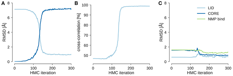
Figure 1. Flexible fitting of adenylate kinase into a 10 Å map. (A) Evolution of the RMSD to the initial structure (4ake) shown in dark blue and the target structure (1ake) shown in light blue. (B) Evolution of the cross-correlation coefficient during flexible fitting. (C) RMSD reduced to Cα atoms that are part of the same rigid domain.
图 1. 腺苷酸激酶在 10 埃地图中的柔性拟合。（A）与初始结构（4ake，深蓝色显示）和目标结构（1ake，浅蓝色显示）的 RMSD 演变。（B）柔性拟合过程中互相关系数的演变。（C）降至同一刚性域内的 Cα原子的 RMSD。

3.2. Flexible Fitting Benchmark
3.2. 灵活拟合基准

To systematically validate local flexible fitting of EM maps with ISD, I applied HMC sampling of the posterior distribution to a benchmark proposed by Topf et al. (2008) to test their Flex-EM method. The Flex-EM benchmark comprises various medium sized proteins and simulated EM maps at different resolutions ranging from 4 to 14 Å. For each flexible fitting task of the single-domain subset, I launched an HMC sampler starting from the initial structure as provided by the benchmark. The initial structure was obtained by homology modeling based on a template structure that shows an alternative conformational state. The task is to deform the homology model such that it better agrees with a simulated EM map showing a different conformational state.
为了系统地验证 EM 图谱与 ISD 的局部灵活拟合，我应用了 HMC 采样对 Topf 等人（2008 年）提出的基准测试中的后验分布进行了采样，以测试他们的 Flex-EM 方法。Flex-EM 基准测试包括各种中等大小的蛋白质和不同分辨率（从 4 到 14 埃）的模拟 EM 图谱。对于单域子集的每个灵活拟合任务，我都从基准测试提供的初始结构开始启动 HMC 采样器。初始结构是通过对显示不同构象状态的模板结构进行同源建模获得的。任务是将同源模型变形，使其更好地与显示不同构象状态的模拟 EM 图谱一致。

Figure 2 shows the results of a flexible fitting benchmark from Topf et al. (2008). In all cases, ISD improves the fit of the initial structure quite significantly and achieves cross-correlation coefficients above 95%. Moreover, the RMSDs of the final structures fitted with ISD are systematically better than the fits obtained with Flex-EM.
图 2 显示了 Topf 等人（2008 年）的一个灵活拟合基准测试的结果。在所有情况下，ISD 都显著改善了初始结构的拟合度，并实现了 95%以上的互相关系数。此外，使用 ISD 拟合的最终结构的 RMSD 系统地优于使用 Flex-EM 获得的拟合度。

FIGURE 2  图 2

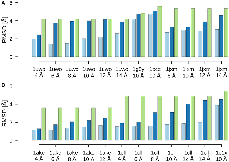
Figure 2. Flexible fitting benchmark. Shown are the RMSD values for the final results of flexible fitting with ISD (light blue) and Flex-EM (dark blue) in comparison to the RMSD of the initial structure to the target structure (green). (A) Flexible fitting results for 1uwo, 1g5y, 1ccz, 1jxm. (B) Flexible fitting results for 1ake, 1cll, 1c1x.
图 2. 灵活拟合基准。显示了使用 ISD（浅蓝色）和 Flex-EM（深蓝色）进行灵活拟合的最终结果的 RMSD 值，与初始结构到目标结构的 RMSD（绿色）进行了比较。（A）1uwo、1g5y、1ccz、1jxm 的灵活拟合结果。（B）1ake、1cll、1c1x 的灵活拟合结果。

Although flexible fitting with HMC performs well in practice, there are still conceptual problems with this approach. Sampling with HMC does not explore the full posterior distribution, but stays in the vicinity of the initial structure. A truly Bayesian approach, however, aims to explore the entire posterior distribution by using, for example, a full-blown replica simulation. However, global sampling of the posterior will result in many alternative fits of the EM map that will show a large RMSD to the target structure, because the force fields implemented in ISD cannot distinguish between the target structure and other globular structures that fit the density map. A remedy is to not only use the known structure that is fitted against the EM map as the initial structure, but also to develop a probabilistic model that allows for deformations of the known structure. Such a model is currently under development.
尽管使用 HMC 进行灵活拟合在实践中表现良好，但这种方法仍然存在概念上的问题。HMC 采样并没有探索整个后验分布，而是停留在初始结构的附近。然而，一个真正的贝叶斯方法旨在通过使用例如完全复制的模拟来探索整个后验分布。然而，对后验的全局采样将导致许多替代的 EM 图拟合，这些拟合与目标结构将显示出较大的 RMSD，因为 ISD 中实现的力场无法区分目标结构和其他适合密度图的球形结构。解决方法是不仅使用与 EM 图拟合的已知结构作为初始结构，而且还要开发一个允许已知结构变形的概率模型。这样的模型目前正在开发中。

3.3. Global Fitting of Symmetric Assemblies
3.3. 全局拟合对称组件

Global sampling of the posterior distribution is currently only possible in ISD, if the internal structure of the subunits is kept fixed. The only degrees of freedom are the six external degrees of freedom parameterizing a global rotation and translation of each subunit. The sampling problem arising in global fitting of EM maps is quite severe. To see this, let us first study sampling from the prior (Equation 12), which is the Boltzmann ensemble confined by a soft box containing the experimental density map. Sampling from this prior is a sort of toy version of the density fitting problem. Instead of fitting the assembly against the density map, our aim is to generate non-clashing configurations that lie inside a box which contains the thresholded map. This is an instance of a 3D packing problem, which is NP-hard.
目前，只有在 ISD 中，如果子单元的内部结构保持固定，才可能对后验分布进行全局采样。唯一的自由度是参数化每个子单元全局旋转和平移的六个外部自由度。在全局拟合 EM 图谱中出现的采样问题相当严重。为了看到这一点，让我们首先研究从先验（方程 12）中采样，该先验是由包含实验密度图的软盒子限制的玻尔兹曼集合。从这个先验中采样是密度拟合问题的一种玩具版本。我们的目标不是将组装体与密度图进行拟合，而是生成位于包含阈值图的盒子内的非冲突配置。这是一个 3D 装箱问题的实例，它是 NP 难的。

Let us look at a specific example: The symmetric chaperonin GroEL has been studied extensively by cryo-EM, X-ray crystallography and NMR. A 3D reconstruction of GroEL at a resolution of 4.1 Å is available (EMD-6422). The original map spans 240³ voxels. The EMDB entry suggests a user-defined threshold of ρ_min = 3.5 for visualizing the map. After thresholding (Equation 10) and cropping, the grid has 135 × 133 × 133 voxels, i.e., only ~ 17% of the original volume carries information that is useful for structural modeling. The 3D cropping operation results in a box that spans a volume of 144.5 × 142.3 × 142.3 ų. This example illustrates that thresholding and cropping can achieve a drastic reduction in the number of grid points that have to be evaluated during density fitting.
让我们看一个具体的例子：对称性伴侣蛋白 GroEL 已经通过冷冻电子显微镜、X 射线晶体学和核磁共振广泛研究。GroEL 的 3D 重建图分辨率为 4.1 埃（EMD-6422）。原始图谱跨越了 240 个体素。EMDB 条目建议一个用户定义的阈值ρ=3.5 来可视化图谱。经过阈值化（方程 10）和裁剪后，网格有 135×133×133 个体素，即只有大约 17%的原始体积包含有用于结构建模的信息。3D 裁剪操作导致一个跨越 144.5×142.3×142.3 埃体积的盒子。这个例子说明了阈值化和裁剪可以在密度拟合过程中大幅度减少必须评估的网格点数量。

GroEL exhibits a seven-fold tetrahedral symmetry (D7). Therefore, our task is to sample configurations of the 14-mer that fit inside the box and minimize the overlap between atoms from different subunits. I used a Tsallis replica simulation to sample structures of the GroEL 14-mer. There are only six conformational degrees of freedom: three rotational and three translational degrees of freedom, which determine the position and orientation of a single GroEL subunit. The positions and orientations of the other 13 subunits are generated by the action of the D7 symmetry operator.
GroEL 表现出七重四面体对称性（D7）。因此，我们的任务是采样适合在盒子内的 14 聚体构象，并最小化不同亚基之间原子的重叠。我使用了 Tsallis 复制模拟来采样 GroEL 14 聚体的结构。只有六个构象自由度：三个旋转自由度和三个平移自由度，这些决定了单个 GroEL 亚基的位置和方向。其他 13 个亚基的位置和方向是通过 D7 对称操作符的作用生成的。

Although this is a low-dimensional sampling problem, it turns out to be surprisingly hard. I needed 59 replicas in the Tsallis ensemble to achieve an average swap rate of 38%. If the non-bonded interactions are fully switched on, there are only few arrangements that fit into the box without producing significant clashes between atoms from different subunits. As a consequence, the box prior exhibits a few isolated peaks. The shape of the prior distribution is reminiscent of a golf-course energy landscape and quite different from the funnel-shaped energy landscape imposed by distance restraints.
尽管这是一个低维采样问题，但事实证明它出奇地难以解决。我需要在 Tsallis 系综中使用 59 个副本才能达到平均交换率 38%。如果完全打开非键合相互作用，只有很少的排列能够适应盒子而不产生不同亚基之间原子的显著冲突。因此，盒子先验表现出几个孤立的峰值。先验分布的形状让人联想到高尔夫球场的能量景观，与距离约束强加的漏斗形能量景观截然不同。

Clustering of the sampled rigid-body degrees of freedom yields six groups of symmetric assemblies that fit into the box (see Figure 3 and Table 1). Each group is defined very precisely with an ensemble RMSD ranging between 0.13 and 0.23 Å over the entire 14-mer. The tightness of the clusters shows that there is only a discrete set of arrangements that fits into the box. The first three clusters achieve the lowest non-bonded energies E(θ). The energy of the next two clusters is elevated by 70 units. Replica-exchange Monte Carlo occasionally also samples a high-energy structure (cluster 6). The first five clusters show the same arrangement of the seven-membered ring formed by chains A–G. The RMSD of these chains to the arrangement in the crystal structure is below 0.8 Å; only the last cluster shows a higher RMSD of 4.7 Å. The major difference between the clusters is in how the rings are arranged relative to each other. In clusters 1, 2, 3, and 6, the two rings are oriented in the same fashion as in the crystal structure (with the termini facing each other), whereas clusters 4 and 5 show an inverted orientation.
对采样的刚体自由度进行聚类，得到六组对称组装体，它们适合放入盒子中（见图 3 和表 1）。每组都定义得非常精确，整个 14 聚体的集合 RMSD 在 0.13 到 0.23 埃之间。簇的紧密度表明，只有一组离散的排列适合放入盒子中。前三簇达到了最低的非键合能量 E(θ)。接下来两簇的能量提高了 70 个单位。复制交换蒙特卡洛偶尔也会采样到一个高能结构（簇 6）。前五簇显示了由 A-G 链形成的七元环的相同排列。这些链与晶体结构中的排列的 RMSD 低于 0.8 埃；只有最后一簇显示出较高的 RMSD 为 4.7 埃。簇之间的主要区别在于环相对于彼此的排列方式。在簇 1、2、3 和 6 中，两个环的取向与晶体结构中的相同（末端相对），而簇 4 和 5 显示出相反的取向。

FIGURE 3  图 3

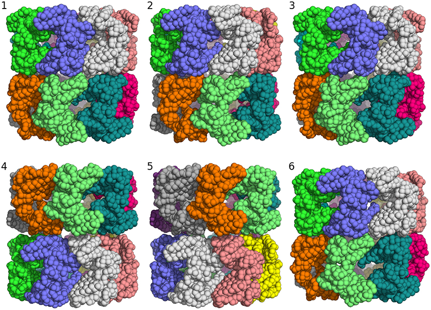
Figure 3. Major structural clusters of the GroEL 14-mer generated from the prior distribution confined to a box. Subunits are color coded. The lowest energy clusters are shown on top (structures 1–3). The second lowest energy structures are clusters 4 and 5. Structure 6 is a rare high energy configuration that is also generated by replica-exchange Monte Carlo.
图 3. 从限制在盒子内的先验分布生成的 GroEL 14 聚体的主要结构簇。亚基按颜色编码。最低能量簇显示在顶部（结构 1-3）。第二低能量结构是簇 4 和 5。结构 6 是一种罕见的高能构象，也是通过复制交换蒙特卡洛生成的。

TABLE 1  表 1

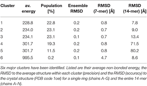
Table 1. Summary of a clustering analysis of the prior ensemble of GroEL.
表 1. GroEL 先验集合聚类分析摘要。

Posteriors based on distance data such as those arising in NMR applications exhibit a continuum of high-probability structures. The Markov chain is guided to the most likely structures by a funnel-shaped probability landscape. The distributions arising in EM fitting problems show a very different landscape with multiple isolated peaks that carry similar probability mass and therefore all contribute significantly to the posterior. Rigid-body modeling with EM maps can be viewed as a 3D packing problem. In case of GroEL, the packing constraint from the prior box and the D7 symmetry already determine the overall structure of the assembly to a large degree without any use of the density map. But the tests also show that even sampling from the prior alone can be quite challenging.
基于距离数据的后验，如在 NMR 应用中出现的，展示了一个高概率结构的连续体。马尔可夫链通过一个漏斗形的概率景观被引导至最可能的结构。在 EM 拟合问题中出现的分布展示了一个非常不同的景观，有多个孤立的峰值携带相似的概率质量，因此都对后验有显著贡献。使用 EM 图的刚体建模可以被视为一个 3D 装箱问题。在 GroEL 的情况下，先验盒子的装箱约束和 D7 对称性已经在很大程度上决定了组装的整体结构，而无需使用密度图。但测试也表明，即使仅从先验中采样也可能相当具有挑战性。

The minimum energy assembly sampled from the prior fits the density map only poorly with a cross-correlation of ~10%. Refining the assembly in the presence of the map improves the cross-correlation to 55% and decreases the RMSD of the entire 14-mer to 1.1 Å.
从先验中采样的最小能量组装与密度图的互相关仅为~10%，在图谱存在的情况下对组装进行精细化可以提高互相关至 55%，并将整个 14 聚体的 RMSD 降低到 1.1 埃。

3.4. Multi-Body Modeling of GroEL/ES
3.4. GroEL/ES 的多体建模

In general rigid-body modeling applications, we have to fit multiple rigid bodies into an EM map. I will use the GroEL/ES complex to illustrate multi-body fitting with ISD. GroEL/ES is formed by GroEL and the cochaperonin GroES. GroES interacts with one of the seven-membered rings formed by GroEL after a conformational change has been induced in the subunits. Therefore, the structures of the two GroEL 7-mers are no longer identical, and we have to fit three rigid bodies: one subunit of free GroEL (PDB code 1aon, chain A), one subunit of GroEL in complex with GroES (1aon, chain H), and one subunit of GroES (1aon, chain O). Each of the three subunits is duplicated by the action of a 7-fold cyclic symmetry. The symmetry mates are not represented explicitly, but generated from each of the three rigid bodies. Forces that act on the symmetry mates are backprojected onto the subunit. Therefore, we have a total of 18 conformational degrees of freedom.
在一般的刚体建模应用中，我们需要将多个刚体拟合到 EM 图中。我将使用 GroEL/ES 复合物来说明使用 ISD 的多体拟合。GroEL/ES 由 GroEL 和辅蛋白 GroES 组成。GroES 在与 GroEL 的七个亚基环中的一个发生构象变化后与其相互作用。因此，两个 GroEL 七聚体的结构不再相同，我们必须拟合三个刚体：一个自由 GroEL 的亚基（PDB 代码 1aon，链 A），一个与 GroES 复合物中的 GroEL 亚基（1aon，链 H），以及一个 GroES 亚基（1aon，链 O）。这三个亚基每一个都通过 7 重循环对称性的作用而被复制。对称配体没有明确表示，而是从每个刚体生成。作用在对称配体上的力被反投影到亚基上。因此，我们总共有 18 个构象自由度。

I used ISD to fit GroEL/ES into a 23.5 Å map (Ranson et al., 2001) (EMD-1046). To shortcut the convergence of posterior sampling, I first ran a replica simulation with a Cα representation of the subunits and switched off the non-bonded interactions. With this strategy, the sampler rapidly generates models that achieve a cross-correlation of 96% (see Figure 4D). Inspection of the structures shows that there are two clusters which differ only in the structure of the GroES subunit. The structure of the two GroEL rings is already very close to the crystal structure (1aon) with an RMSD of 3.5 ± 0.5 Å over the 14-mer formed by the GroEL subunits (Figure 4A). The GroES 7-mer arranges in two versions of the ring: One is the correct structure with an RMSD of 2.1 ± 0.6 Å to the crystal structure. The second structure is incorrect with an RMSD of 20.0 ± 0.3 Å. Both structures are almost equally populated. The correct structure is adopted by 51.3% of the structures; the population of the incorrect assembly is 47.7% (see Figure 4B). There is a tiny fraction with a population of ~1% that shows a third arrangement of the GroES subunit (RMSD 9.17 ± 0.51 Å). Figure 4C shows the distribution of the RMSD over the entire assembly.
我使用 ISD 将 GroEL/ES 拟合到 23.5 Å的地图中（Ranson 等人，2001 年）（EMD-1046）。为了加快后验采样的收敛速度，我首先运行了一个具有亚基 Cα表示的复制模拟，并关闭了非键合相互作用。采用这种策略，采样器迅速生成了达到 96%交叉相关性的模型（见图 4D）。结构检查显示有两个簇，它们仅在 GroES 亚基的结构上有所不同。两个 GroEL 环的结构已经非常接近晶体结构（1aon），在由 GroEL 亚基形成的 14 聚体上的 RMSD 为 3.5 ± 0.5 Å（见图 4A）。GroES 7 聚体以两种环的版本排列：一个是与晶体结构 RMSD 为 2.1 ± 0.6 Å的正确结构。第二个结构是不正确的，RMSD 为 20.0 ± 0.3 Å。这两种结构几乎同样丰富。正确结构被 51.3%的结构采用；错误组装的种群为 47.7%（见图 4B）。有大约 1%的极小部分显示了 GroES 亚基的第三种排列（RMSD 9.17 ± 0.51 Å）。 图 4C 显示了整个组装体上 RMSD 的分布。

FIGURE 4  图 4

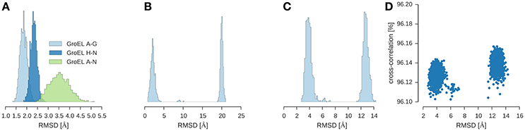
Figure 4. Multi-body modeling of GroEL/ES. Shown is the RMSD between structural models obtained by posterior sampling with ISD and the crystal structure (PDB code 1aon). (A) RMSD for GroEL subunits for both 7-membered rings (chains A–G and chains H–N) and for the entire 14-mer (chains A–N). (B) RMSD for GroES (chains O–U) (C) RMSD for the entire 21-mer. (D) Correlation between the overall RMSD (21-mer) and the cross-correlation coefficient.
图 4. GroEL/ES 的多体建模。显示了通过 ISD 后采样获得的结构模型与晶体结构（PDB 代码 1aon）之间的 RMSD。（A）GroEL 亚基的 RMSD，对于 7 元环（链 A-G 和链 H-N）以及整个 14 聚体（链 A-N）。（B）GroES 的 RMSD（链 O-U）（C）整个 21 聚体的 RMSD。（D）整体 RMSD（21 聚体）与交叉相关系数之间的相关性。

In a refinement step, I used a full-atom representation of the subunits and switched on the non-bonded energy terms. The RMSD to the crystal structure drops to 1.4 Å without compromising the fit to the EM map: the cross-correlation coefficient of the full-atom structure is still 96%.
在细化步骤中，我使用了亚基的全原子表示，并打开了非键合能量项。与晶体结构的 RMSD 降低到 1.4 埃，同时不影响与电子显微图的拟合：全原子结构的互相关系数仍为 96%。

3.5. Estimation of the Precision of an EM Map
3.5. EM 图精度的估计

As outlined in Section 2.2.1, it is challenging to obtain a good estimate of the precision of an EM map, because an EM map typically contains many zero-density voxels in addition to the non-noise voxels, but only voxels carrying a real signal should contribute to the precision. To identify which voxels carry true signal, we would have to first solve the fitting problem. Therefore, both problems, the estimation of a well-fitting structure and the construction of a good mask, are highly related. Moreover, the errors (i.e., the discrepancy between the experimental and calculated maps) are spatially correlated, but the Gaussian model (3) treats them as completely independent observations, which also results in an artificial increase in the precision. The reason for the latter effect is the following: If errors are correlated, the effective number of data points is smaller than the number of voxels (Sivia, 2004). According to Equation (7) the precision of the map is proportional to the number of voxels for the simple Gaussian model, the precision will therefore be overestimated, if the errors between neighboring voxels are correlated.
正如 2.2.1 节所述，要获得 EM 图精度的良好估计是具有挑战性的，因为 EM 图通常包含许多零密度体素以及非噪声体素，但只有携带真实信号的体素才应该对精度有所贡献。为了识别哪些体素携带真实信号，我们首先必须解决拟合问题。因此，两个问题，即拟合结构的估计和构建良好的掩模，都是高度相关的。此外，误差（即实验图和计算图之间的差异）在空间上是相关的，但高斯模型（3）将它们视为完全独立的观测值，这也导致了精度的人为增加。后一效应的原因是：如果误差是相关的，有效数据点的数量小于体素的数量（Sivia, 2004）。根据方程（7），对于简单的高斯模型，图的精度与体素数量成正比，因此，如果相邻体素之间的误差是相关的，精度将被高估。

Let us illustrate the various factors that influence the precision for a concrete example. Figure 5 shows the distribution of the discrepancy between the experimental and the calculated density map for the GroEL/ES map analyzed in the previous section. The Gaussian likelihood assumes that this distribution has a bell-shaped curve whose width is determined by the precision λ. The distribution of the discrepancy ϵ_n = ρ_n − ρ(x_n; θ, σ) is shown in (Figures 5A–D) for various stages of preprocessing. The original map contains many low-density voxels that lead to a very sharp, dominating peak at zero in the distribution of ϵ_n (Figure 5A). Cropping (Figure 5B) and subsequent decimation (Figure 5C) chops away many of the zero-density voxels and decreases the detrimental effect of the low-density voxels. However, the distribution of ϵ_n is only captured well by a Gaussian, if we mask out low-density voxels (see Figure 5D). The effect of the preprocessing steps on the estimated precision is shown in Figure 5E. Each of the preparation steps lowers the estimated precision by orders of magnitude.
让我们通过一个具体的例子来说明影响精度的各种因素。图 5 显示了前一节分析的 GroEL/ES 图谱实验密度图与计算密度图之间差异的分布。高斯似然假设这个分布有一个钟形曲线，其宽度由精度λ决定。差异分布ϵ _n = ρ _n − ρ(x _n ; θ, σ)在（图 5A-D）中展示了不同预处理阶段的情况。原始图谱包含许多低密度体素，导致ϵ _n 分布中零点处有一个非常尖锐的主峰（图 5A）。裁剪（图 5B）和随后的抽取（图 5C）去除了许多零密度体素，并减少了低密度体素的不良影响。然而，如果我们屏蔽掉低密度体素，ϵ _n 的分布才能很好地用高斯分布来捕捉（见图 5D）。预处理步骤对估计精度的影响如图 5E 所示。每一个准备步骤都将估计精度降低了数个数量级。

FIGURE 5  图 5

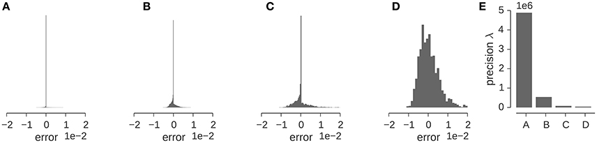
Figure 5. Estimation of the precision λ of the GroEL/ES map. (A–D) Show the distribution of the “error” (or discrepancy) between the experimental and calculated maps ρ_n − ρ(x_n; θ, σ). Error distribution for the full map (A), full map after cropping (B), the downsampled and cropped map (C), the downsampled, cropped and masked map (D). (E) Estimated precision for the different input maps used in multi-body fitting.
图 5. GroEL/ES 图谱精度λ的估计。（A-D）展示了实验图谱ρ _n 与计算图谱ρ(x _n ; θ, σ)之间的“误差”（或差异）分布。全图谱的误差分布（A），裁剪后的全图谱（B），下采样并裁剪的图谱（C），下采样、裁剪并掩膜的图谱（D）。（E）多体拟合中使用的不同输入图谱的估计精度。

4. Conclusion  4. 结论

This article discusses how ISD incorporates EM maps into a structure calculation and demonstrates some aspects of Bayesian integrative modeling with EM data. The Bayesian framework is highly suited to address issues in structural modeling with hybrid data such as how to weigh multiple datasets relative to each other. The major bottleneck of an inferential structure determination is conformational sampling. The posterior distribution arising in EM fitting poses a challenging sampling problem, which can be overcome with replica-exchange Monte Carlo.
本文讨论了 ISD 如何将 EM 图谱纳入结构计算，并展示了使用 EM 数据进行贝叶斯整合建模的一些方面。贝叶斯框架非常适合解决混合数据结构建模中的问题，例如如何相对权衡多个数据集。推断结构确定的主要瓶颈是构象采样。EM 拟合中出现的后验分布提出了一个具有挑战性的采样问题，可以通过复制交换蒙特卡洛方法来克服。

The article does not cover crosslinking/mass spectrometry and solid-state NMR, which are complementary methods for characterizing the structure of large assemblies. ISD has also been used to model biomolecular assemblies from solid-state NMR data. For example, we have used ISD to compute the structure of the membrane domain of the trimeric autotransporter adhesin YadA (Shahid et al., 2012). We modeled a fully flexible subunit in the presence of a cyclic trimer symmetry. Although the data are highly ambiguous due to the imprecision of solid-state NMR restraints and the trimer symmetry, ISD was able to determine the correct structure of the YadA membrane anchor domain. Another example is our recent structure of a type 1 pilus FimA from E. coli (Habenstein et al., 2015). Here solid-state NMR and scanning electron microscopy data were combined with solution NMR data to estimate the internal structure of the subunit as well as the parameters of the helical symmetry of the FimA pilus. Also modeling with crosslinking data is possible with ISD, e.g., Carstens et al. (2016) discuss chromosome structure modeling. However, the use of crosslinking data for modeling macromolecular complexes still needs to be benchmarked thoroughly. A common scenario is to combine cryo-EM with crosslinking data, which also needs to be tested systematically with ISD. A Bayesian approach to modeling macromolecular assemblies with crosslinking data has been proposed recently by Ferber et al. (2016).
本文未涉及交联/质谱和固态核磁共振，这些是表征大型组装体结构的补充方法。ISD 也被用来从固态核磁共振数据模拟生物分子组装体。例如，我们使用 ISD 计算了三聚体自转运粘附素 YadA 的膜结构域（Shahid 等人，2012 年）。我们在环状三聚体对称性的存在下模拟了一个完全灵活的亚基。尽管由于固态核磁共振约束的不精确性和三聚体对称性，数据高度模糊，ISD 仍能够确定 YadA 膜锚定域的正确结构。另一个例子是我们最近对大肠杆菌 I 型菌毛 FimA 的结构研究（Habenstein 等人，2015 年）。在这里，固态核磁共振和扫描电子显微镜数据与溶液核磁共振数据相结合，以估计亚基的内部结构以及 FimA 菌毛螺旋对称性的参数。ISD 也可以用交联数据进行建模，例如，Carstens 等人（2016 年）讨论了染色体结构建模。 然而，使用交联数据对大分子复合物进行建模仍需彻底基准测试。一个常见的场景是将冷冻电镜与交联数据结合起来，这也需要与 ISD 系统地测试。Ferber 等人（2016 年）最近提出了一种使用交联数据对大分子组装进行建模的贝叶斯方法。

Future work will focus on various aspects of modeling with hybrid data. One goal is to develop a better model for EM maps that incorporates the various preprocessing steps discussed in Section 2.2.2. The model will incorporate a mask that will be estimated along with the other unknown parameters. Moreover, we will develop a likelihood function that accounts for spatial correlations between errors in the density map. Another goal is to support modeling with coarse-grained representations of biomolecular systems (Tozzini, 2005; Saunders and Voth, 2013). Especially, for very large systems it will be critical to work with a multiscale representation to enable exhaustive conformational sampling. We are already using highly coarse-grained models for modeling the 3D structure of chromosomes and genomes from chromosome conformation capture data (Carstens et al., 2016).
未来的工作将集中在使用混合数据建模的各个方面。一个目标是开发一个更好的电子显微镜（EM）图谱模型，该模型将结合第 2.2.2 节讨论的各种预处理步骤。该模型将包含一个掩模，该掩模将与其它未知参数一起估计。此外，我们将开发一个考虑密度图误差之间空间相关性的似然函数。另一个目标是支持使用生物分子系统的粗粒度表示进行建模（Tozzini, 2005; Saunders and Voth, 2013）。特别是，对于非常大的系统，使用多尺度表示进行工作将是至关重要的，以实现详尽的构象采样。我们已经在使用高度粗粒度的模型来建模来自染色体构象捕获数据的染色体和基因组的 3D 结构（Carstens et al., 2016）。

Author Contributions  作者贡献

MH designed and performed research and wrote the manuscript.
MH 设计并执行研究，并撰写了手稿。

Funding  资金

The author acknowledges funding from the German Research Foundation (DFG) (SFB 860, Project B09).
作者感谢德国研究基金会（DFG）（SFB 860，项目 B09）的资助。

Conflict of Interest Statement
利益冲突声明

The author declares that the research was conducted in the absence of any commercial or financial relationships that could be construed as a potential conflict of interest.
作者声明本研究是在没有任何可能被解释为潜在利益冲突的商业或财务关系的情况下进行的。

References  参考文献

Agafonov, D. E., Kastner, B., Dybkov, O., Hofele, R. V., Liu, W. T., Urlaub, H., et al. (2016). Molecular architecture of the human U4/U6.U5 tri-snRNP. Science 351, 1416–1420. doi: 10.1126/science.aad2085
阿加福诺夫，D. E.，卡斯纳，B.，迪布科夫，O.，霍费勒，R. V.，刘文涛，W. T.，乌拉布，H. 等。（2016）。人类 U4/U6.U5 三小核 RNA 复合体的分子架构。科学 351, 1416–1420. doi: 10.1126/science.aad2085

PubMed Abstract | CrossRef Full Text | Google Scholar
PubMed 摘要 | CrossRef 全文 | Google Scholar

Anger, A. M., Armache, J. P., Berninghausen, O., Habeck, M., Subklewe, M., Wilson, D. N., et al. (2013). Structures of the human and Drosophila 80S ribosome. Nature 497, 80–85. doi: 10.1038/nature12104
愤怒，A. M.，Armache，J. P.，Berninghausen，O.，Habeck，M.，Subklewe，M.，Wilson，D. N.等。（2013）。人类和果蝇 80S 核糖体的结构。自然 497，80-85。doi：10.1038/nature12104

PubMed Abstract | CrossRef Full Text | Google Scholar

Bai, X. C., Yan, C., Yang, G., Lu, P., Ma, D., Sun, L., et al. (2015). An atomic structure of human γ-secretase. Nature 525, 212–217. doi: 10.1038/nature14892

PubMed Abstract | CrossRef Full Text | Google Scholar

Bayrhuber, M., Meins, T., Habeck, M., Becker, S., Giller, K., Villinger, S., et al. (2008). Structure of the human voltage-dependent anion channel. Proc. Natl. Acad. Sci. U.S.A. 105, 15370–15375. doi: 10.1073/pnas.0808115105

PubMed Abstract | CrossRef Full Text | Google Scholar

Beckstein, O., Denning, E. J., Perilla, J. R., and Woolf, T. B. (2009). Zipping and unzipping of adenylate kinase: atomistic insights into the ensemble of open closed transitions. J. Mol. Biol. 394, 160–176. doi: 10.1016/j.jmb.2009.09.009

PubMed Abstract | CrossRef Full Text | Google Scholar

Berman, H. M., Westbrook, J., Feng, Z., Gilliland, G., Bhat, T. N., Weissig, H., et al. (2000). The protein data bank. Nucleic Acids Res. 28, 235–242. doi: 10.1093/nar/28.1.235

PubMed Abstract | CrossRef Full Text | Google Scholar

Bernardo, J. M., and Smith, A. F. M. (2009). Bayesian Theory. Wiley Series in Probability and Statistics. New York, NY: John Wiley & Sons.

Google Scholar

Brünger, A. T. (1992). The free R value: a novel statistical quantity for assessing the accuracy of crystal structures. Nature 355, 472–474.

PubMed Abstract | Google Scholar

Brünger, A. T., and Nilges, M. (1993). Computational challenges for macromolecular structure determination by X-ray crystallography and solution NMR spectroscopy. Q. Rev. Biophys. 26, 49–125. doi: 10.1017/S0033583500003966

PubMed Abstract | CrossRef Full Text | Google Scholar

Carstens, S., Nilges, M., and Habeck, M. (2016). Inferential structure determination of chromosomes from single-cell Hi-C data. PLoS Comput. Biol. 12:e1005292. doi: 10.1371/journal.pcbi.1005292

PubMed Abstract | CrossRef Full Text | Google Scholar

Chiu, W., Baker, M. L., Jiang, W., Dougherty, M., and Schmid, M. F. (2005). Electron cryomicroscopy of biological machines at subnanometer resolution. Structure 13, 363–372. doi: 10.1016/j.str.2004.12.016

PubMed Abstract | CrossRef Full Text | Google Scholar

Cox, R. T. (1946). Probability, frequency and reasonable expectation. Am. J. Phys. 14, 1–13. doi: 10.1119/1.1990764

CrossRef Full Text | Google Scholar

Delarue, M., and Dumas, P. (2004). On the use of low-frequency normal modes to enforce collective movements in refining macromolecular structural models. Proc. Natl. Acad. Sci. U.S.A. 101, 6957–6962. doi: 10.1073/pnas.0400301101

PubMed Abstract | CrossRef Full Text | Google Scholar

Devroye, L. (1986). Non-uniform Random Variate Generation. New York, NY: Springer Verlag.

Google Scholar

DiMaio, F., Tyka, M. D., Baker, M. L., Chiu, W., and Baker, D. (2009). Refinement of protein structures into low-resolution density maps using rosetta. J. Mol. Biol. 392, 181–190. doi: 10.1016/j.jmb.2009.07.008

PubMed Abstract | CrossRef Full Text | Google Scholar

Duane, S., Kennedy, A. D., Pendleton, B., and Roweth, D. (1987). Hybrid Monte Carlo. Phys. Lett. B 195, 216–222. doi: 10.1016/0370-2693(87)91197-X

CrossRef Full Text | Google Scholar

Earl, D. J., and Deem, M. W. (2005). Parallel tempering: theory, applications, and new perspectives. Phys. Chem. Chem. Phys. 7, 3910–3916. doi: 10.1039/b509983h

PubMed Abstract | CrossRef Full Text | Google Scholar

Esquivel-Rodríguez, J., and Kihara, D. (2013). Computational methods for constructing protein structure models from 3D electron microscopy maps. J. Struct. Biol. 184, 93–102. doi: 10.1016/j.jsb.2013.06.008

PubMed Abstract | CrossRef Full Text | Google Scholar

Fabiola, F., and Chapman, M. S. (2005). Fitting of high-resolution structures into electron microscopy reconstruction images. Structure 13, 389–400. doi: 10.1016/j.str.2005.01.007

PubMed Abstract | CrossRef Full Text | Google Scholar

Ferber, M., Kosinski, J., Ori, A., Rashid, U. J., Moreno-Morcillo, M., Simon, B., et al. (2016). Automated structure modeling of large protein assemblies using crosslinks as distance restraints. Nat. Methods 13, 515–520. doi: 10.1038/nmeth.3838

PubMed Abstract | CrossRef Full Text | Google Scholar

Fischer, N., Neumann, P., Konevega, A. L., Bock, L. V., Ficner, R., Rodnina, M. V., et al. (2015). Structure of the E. coli ribosome-EF-Tu complex at <3 Å resolution by Cs-corrected cryo-EM. Nature 520, 567–570. doi: 10.1038/nature14275

PubMed Abstract | CrossRef Full Text | Google Scholar

Frank, J. (2002). Single-particle imaging of macromolecules by cryo-electron microscopy. Annu. Rev. Biophys. Biomol. Struct. 31, 303–319. doi: 10.1146/annurev.biophys.31.082901.134202

PubMed Abstract | CrossRef Full Text | Google Scholar

Galej, W. P., Wilkinson, M. E., Fica, S. M., Oubridge, C., Newman, A. J., and Nagai, K. (2016). Cryo-EM structure of the spliceosome immediately after branching. Nature 537, 197–201. doi: 10.1038/nature19316

PubMed Abstract | CrossRef Full Text | Google Scholar

Gallego, G., and Yezzi, A. (2015). “A compact formula for the derivative of a 3-d rotation in exponential coordinates”. J. Math. Imaging Vis. 51, 378–384. doi: 10.1007/s10851-014-0528-x

CrossRef Full Text | Google Scholar

Geman, S., and Geman, D. (1984). Stochastic relaxation, gibbs distributions, and the Bayesian restoration of images. IEEE Trans. PAMI 6, 721–741. doi: 10.1109/TPAMI.1984.4767596

PubMed Abstract | CrossRef Full Text | Google Scholar

Gerstein, M., Lesk, A. M., and Chothia, C. (1994). Structural mechanisms for domain movements in proteins. Biochemistry 33, 6739–6749. doi: 10.1021/bi00188a001

PubMed Abstract | CrossRef Full Text | Google Scholar

Geyer, C. J. (1991). “Markov chain Monte Carlo maximum likelihood,” in Computing Science and Statistics: Proceedings of the 23rd Symposium on the Interface (Fairfax Station, VA: Interface Foundation of North America), 156–163.

Google Scholar

Gingras, A. C., Gstaiger, M., Raught, B., and Aebersold, R. (2007). Analysis of protein complexes using mass spectrometry. Nat. Rev. Mol. Cell Biol. 8, 645–654. doi: 10.1038/nrm2208

PubMed Abstract | CrossRef Full Text | Google Scholar

Habeck, M. (2011). Statistical mechanics analysis of sparse data. J. Struct. Biol. 173, 541–548. doi: 10.1016/j.jsb.2010.09.016

PubMed Abstract | CrossRef Full Text | Google Scholar

Habeck, M. (2012). “Inferential structure determination from nmr data,” in Bayesian Methods in Structural Bioinformatics eds T. Hamelryck, K. Mardia, and J. Ferkinghoff-Borg (Berlin; Heidelberg: Springer), 287–311. doi: 10.1007/978-3-642-27225-7_12

CrossRef Full Text | Google Scholar

Habeck, M., Nilges, M., and Rieping, W. (2005a). Bayesian inference applied to macromolecular structure determination. Phys. Rev. E 72:031912. doi: 10.1103/PhysRevE.72.031912

PubMed Abstract | CrossRef Full Text | Google Scholar

Habeck, M., Nilges, M., and Rieping, W. (2005b). Replica-exchange Monte Carlo scheme for Bayesian data analysis. Phys. Rev. Lett. 94, 0181051–0181054. doi: 10.1103/PhysRevLett.94.018105

PubMed Abstract | CrossRef Full Text | Google Scholar

Habeck, M., Rieping, W., and Nilges, M. (2006). Weighting of experimental evidence in macromolecular structure determination. Proc. Natl. Acad. Sci. U.S.A. 103, 1756–1761. doi: 10.1073/pnas.0506412103

PubMed Abstract | CrossRef Full Text | Google Scholar

Habenstein, B., Loquet, A., Hwang, S., Giller, K., Vasa, S. K., Becker, S., et al. (2015). Hybrid structure of the type 1 pilus of uropathogenic Escherichia coli. Angew. Chem. Int. Ed. Engl. 54, 11691–11695. doi: 10.1002/anie.201505065

PubMed Abstract | CrossRef Full Text | Google Scholar

Hinsen, K., Reuter, N., Navaza, J., Stokes, D. L., and Lacapère, J. J. (2005). Normal mode-based fitting of atomic structure into electron density maps: application to sarcoplasmic reticulum Ca-ATPase. Biophys. J. 88, 818–827. doi: 10.1529/biophysj.104.050716

PubMed Abstract | CrossRef Full Text | Google Scholar

Jack, A., and Levitt, M. (1978). Refinement of large structures by simultaneous minimization of energy and R factor. Acta Cryst. Sect. A 34, 931–935. doi: 10.1107/S0567739478001904

CrossRef Full Text | Google Scholar

Jaynes, E. T. (2003). Probability Theory: The Logic of Science. Cambridge: Cambridge University Press.

Google Scholar

Jolley, C. C., Wells, S. A., Fromme, P., and Thorpe, M. F. (2008). Fitting low-resolution cryo-EM maps of proteins using constrained geometric simulations. Biophys. J. 94, 1613–1621. doi: 10.1529/biophysj.107.115949

PubMed Abstract | CrossRef Full Text | Google Scholar

Karaca, E., and Bonvin, A. M. (2013). Advances in integrative modeling of biomolecular complexes. Methods 59, 372–381. doi: 10.1016/j.ymeth.2012.12.004

PubMed Abstract | CrossRef Full Text | Google Scholar

Khatter, H., Myasnikov, A. G., Natchiar, S. K., and Klaholz, B. P. (2015). Structure of the human 80S ribosome. Nature 520, 640–645. doi: 10.1038/nature14427

PubMed Abstract | CrossRef Full Text | Google Scholar

Knuth, K. H., Habeck, M., Malakar, N. K., Mubeen, A. M., and Placek, B. (2015). Bayesian evidence and model selection. Digit. Signal Process. 47, 50–67. doi: 10.1016/j.dsp.2015.06.012

CrossRef Full Text | Google Scholar

Lawson, C. L., Baker, M. L., Best, C., Bi, C., Dougherty, M., Feng, P., et al. (2011). EMDataBank.org: unified data resource for CryoEM. Nucleic Acids Res. 39, D456–D464. doi: 10.1093/nar/gkq880

PubMed Abstract | CrossRef Full Text | Google Scholar

Liu, J. S. (2001). Monte Carlo Strategies in Scientific Computing. New York, NY: Springer.

Google Scholar

MacKay, D. J. C. (2003). Information Theory, Inference, and Learning Algorithms. Cambridge: Cambridge University Press.

Google Scholar

Mechelke, M., and Habeck, M. (2012). Calibration of Boltzmann distribution priors in Bayesian data analysis. Phys. Rev. E 86:066705. doi: 10.1103/PhysRevE.86.066705

PubMed Abstract | CrossRef Full Text | Google Scholar

Mechelke, M., and Habeck, M. (2014). Bayesian weighting of statistical potentials in NMR structure calculation. PLoS ONE 9:e100197. doi: 10.1371/journal.pone.0100197

PubMed Abstract | CrossRef Full Text | Google Scholar

Metropolis, N., Rosenbluth, M., Rosenbluth, A., Teller, A., and Teller, E. (1957). Equation of state calculations by fast computing machines. J. Chem. Phys. 21, 1087–1092. doi: 10.1063/1.1699114

CrossRef Full Text

Müller, C. W., Schlauderer, G. J., Reinstein, J., and Schulz, G. E. (1996). Adenylate kinase motions during catalysis: an energetic counterweight balancing substrate binding. Structure 4, 147–156. doi: 10.1016/S0969-2126(96)00018-4

PubMed Abstract | CrossRef Full Text | Google Scholar

Neal, R. M. (2010) “MCMC using hamiltonian dynamics,” in The Handbook of Markov Chain Monte Carlo eds S. Brooks, A. Gelman, G. L. Jones, and X.-L. Meng (Chapman & Hall/CRC Press), 113–162.

Google Scholar

Orlova, E. V., and Saibil, H. R. (2004). Structure determination of macromolecular assemblies by single-particle analysis of cryo-electron micrographs. Curr. Opin. Struct. Biol. 14, 584–590. doi: 10.1016/j.sbi.2004.08.004

PubMed Abstract | CrossRef Full Text | Google Scholar

Orzechowski, M., and Tama, F. (2008). Flexible fitting of high-resolution x-ray structures into cryoelectron microscopy maps using biased molecular dynamics simulations. Biophys. J. 95, 5692–5705. doi: 10.1529/biophysj.108.139451

PubMed Abstract | CrossRef Full Text | Google Scholar

Pettersen, E. F., Goddard, T. D., Huang, C. C., Couch, G. S., Greenblatt, D. M., Meng, E. C., et al. (2004). UCSF Chimera–a visualization system for exploratory research and analysis. J. Comput. Chem. 25, 1605–1612. doi: 10.1002/jcc.20084

PubMed Abstract | CrossRef Full Text | Google Scholar

Plaschka, C., Larivière, L., Wenzeck, L., Seizl, M., Hemann, M., Tegunov, D., et al. (2015). Architecture of the RNA polymerase II-Mediator core initiation complex. Nature 518, 376–380. doi: 10.1038/nature14229

PubMed Abstract | CrossRef Full Text | Google Scholar

Ranson, N. A., Farr, G. W., Roseman, A. M., Gowen, B., Fenton, W. A., Horwich, A. L., et al. (2001). ATP-bound states of GroEL captured by cryo-electron microscopy. Cell 107, 869–879. doi: 10.1016/S0092-8674(01)00617-1

PubMed Abstract | CrossRef Full Text | Google Scholar

Rappsilber, J. (2011). The beginning of a beautiful friendship: cross-linking/mass spectrometry and modelling of proteins and multi-protein complexes. J. Struct. Biol. 173, 530–540. doi: 10.1016/j.jsb.2010.10.014

PubMed Abstract | CrossRef Full Text | Google Scholar

Rauhut, R., Fabrizio, P., Dybkov, O., Hartmuth, K., Pena, V., Chari, A., et al. (2016). Molecular architecture of the Saccharomyces cerevisiae activated spliceosome. Science 353, 1399–1405. doi: 10.1126/science.aag1906

PubMed Abstract | CrossRef Full Text | Google Scholar

Rieping, W., Habeck, M., and Nilges, M. (2005). Inferential structure determination. Science 309, 303–306. doi: 10.1126/science.1110428

PubMed Abstract | CrossRef Full Text | Google Scholar

Rieping, W., Nilges, M., and Habeck, M. (2008). ISD: a software package for Bayesian NMR structure calculation. Bioinformatics 24, 1104–1105. doi: 10.1093/bioinformatics/btn062

PubMed Abstract | CrossRef Full Text | Google Scholar

Robinson, C. V., Sali, A., and Baumeister, W. (2007). The molecular sociology of the cell. Nature 450, 973–982. doi: 10.1038/nature06523

PubMed Abstract | CrossRef Full Text | Google Scholar

Russel, D., Lasker, K., Webb, B., Velázquez-Muriel, J., Tjioe, E., Schneidman-Duhovny, D., et al. (2012). Putting the pieces together: integrative modeling platform software for structure determination of macromolecular assemblies. PLoS Biol. 10:e1001244. doi: 10.1371/journal.pbio.1001244

PubMed Abstract | CrossRef Full Text | Google Scholar

Sali, A., Glaeser, R., Earnest, T., and Baumeister, W. (2003). From words to literature in structural proteomics. Nature 422, 216–225. doi: 10.1038/nature01513

PubMed Abstract | CrossRef Full Text | Google Scholar

Saunders, M. G., and Voth, G. A. (2013). Coarse-graining methods for computational biology. Annu. Rev. Biophys. 42, 73–93. doi: 10.1146/annurev-biophys-083012-130348

PubMed Abstract | CrossRef Full Text | Google Scholar

Schröder, G. F. (2015). Hybrid methods for macromolecular structure determination: experiment with expectations. Curr. Opin. Struct. Biol. 31, 20–27. doi: 10.1016/j.sbi.2015.02.016

PubMed Abstract | CrossRef Full Text | Google Scholar

Schröder, G. F., Brunger, A. T., and Levitt, M. (2007). Combining efficient conformational sampling with a deformable elastic network model facilitates structure refinement at low resolution. Structure 15, 1630–1641. doi: 10.1016/j.str.2007.09.021

PubMed Abstract | CrossRef Full Text | Google Scholar

Shahid, S. A., Bardiaux, B., Franks, W. T., Krabben, L., Habeck, M., van Rossum, B. J., et al. (2012). Membrane-protein structure determination by solid-state NMR spectroscopy of microcrystals. Nat. Methods 9, 1212–1217. doi: 10.1038/nmeth.2248

PubMed Abstract | CrossRef Full Text | Google Scholar

Sivia, D. S. (2004). “Some thoughts on correlated noise,” in Bayesian Inference and Maximum Entropy Methods in Science and Engineering: 23RD International Workshop on Bayesian Inference and Maximum Entropy Methods in Science and Engineering, vol. 707 (Melville, NY: AIP Publishing), 303–313. doi: 10.1063/1.1751374

CrossRef Full Text | Google Scholar

Swendsen, R. H., and Wang, J.-S. (1986). Replica Monte Carlo simulation of spin glasses. Phys. Rev. Lett. 57, 2607–2609. doi: 10.1103/PhysRevLett.57.2607

PubMed Abstract | CrossRef Full Text | Google Scholar

Tama, F., Miyashita, O., and Brooks, C. L. (2004). Normal mode based flexible fitting of high-resolution structure into low-resolution experimental data from cryo-EM. J. Struct. Biol. 147, 315–326. doi: 10.1016/j.jsb.2004.03.002

PubMed Abstract | CrossRef Full Text | Google Scholar

Tan, R. K., Devkota, B., and Harvey, S. C. (2008). YUP.SCX: coaxing atomic models into medium resolution electron density maps. J. Struct. Biol. 163, 163–174. doi: 10.1016/j.jsb.2008.05.001

PubMed Abstract | CrossRef Full Text | Google Scholar

Topf, M., Lasker, K., Webb, B., Wolfson, H., Chiu, W., and Sali, A. (2008). Protein structure fitting and refinement guided by cryo-EM density. Structure 16, 295–307. doi: 10.1016/j.str.2007.11.016

PubMed Abstract | CrossRef Full Text | Google Scholar

Tozzini, V. (2005). Coarse-grained models for proteins. Curr. Opin. Struct. Biol. 15, 144–150. doi: 10.1016/j.sbi.2005.02.005

PubMed Abstract | CrossRef Full Text | Google Scholar

Trabuco, L. G., Villa, E., Mitra, K., Frank, J., and Schulten, K. (2008). Flexible fitting of atomic structures into electron microscopy maps using molecular dynamics. Structure 16, 673–683. doi: 10.1016/j.str.2008.03.005

PubMed Abstract | CrossRef Full Text | Google Scholar

Vasishtan, D., and Topf, M. (2011). Scoring functions for cryoEM density fitting. J. Struct. Biol. 174, 333–343. doi: 10.1016/j.jsb.2011.01.012

PubMed Abstract | CrossRef Full Text | Google Scholar

Villa, E., and Lasker, K. (2014). Finding the right fit: chiseling structures out of cryo-electron microscopy maps. Curr. Opin. Struct. Biol. 25, 118–125. doi: 10.1016/j.sbi.2014.04.001

PubMed Abstract | CrossRef Full Text | Google Scholar

Wan, R., Yan, C., Bai, R., Huang, G., and Shi, Y. (2016). Structure of a yeast catalytic step I spliceosome at 3.4 resolution. Science 353, 895–904. doi: 10.1126/science.aag2235

PubMed Abstract | CrossRef Full Text | Google Scholar

Ward, A. B., Sali, A., and Wilson, I. A. (2013). Biochemistry. Integrative structural biology. Science 339, 913–915. doi: 10.1126/science.1228565

PubMed Abstract | CrossRef Full Text | Google Scholar

Whitford, P. C., Noel, J. K., Gosavi, S., Schug, A., Sanbonmatsu, K. Y., and Onuchic, J. N. (2009). An all-atom structure-based potential for proteins: bridging minimal models with all-atom empirical forcefields. Proteins 75, 430–441. doi: 10.1002/prot.22253

PubMed Abstract | CrossRef Full Text | Google Scholar

Yan, C., Hang, J., Wan, R., Huang, M., Wong, C. C., and Shi, Y. (2015). Structure of a yeast spliceosome at 3.6-angstrom resolution. Science 349, 1182–1191. doi: 10.1126/science.aac7629

PubMed Abstract | CrossRef Full Text | Google Scholar

Yan, S., Suiter, C. L., Hou, G., Zhang, H., and Polenova, T. (2013). Probing structure and dynamics of protein assemblies by magic angle spinning NMR spectroscopy. Acc. Chem. Res. 46, 2047–2058. doi: 10.1021/ar300309s

PubMed Abstract | CrossRef Full Text | Google Scholar